
안녕하세요, HELLO
오늘은 DeepLearning.AI에서 진행하는 앤드류 응(Andrew Ng) 교수님의 딥러닝 전문화의 마지막이며, 다섯 번째 과정인 "Sequence Models"을 정리하려고 합니다.
"Sequence Models"의 강의를 통해 '시퀀스 모델과 음성 인식, 음악 합성, 챗봇, 기계 번역, 자연어 처리(NLP)' 등을 이해하고, 순환 신경망(RNN)과 GRU 및 LSTM, 트랜스포머 모델에 대해서 배우게 됩니다. 강의는 아래와 같이 구성되어 있습니다.
~ Recurrent Neural Networks
~ Natural Language Processing & Word Embeddings
~ Sequence Models & Attention Mechanism
~ Transformer Network
"Sequence Models" (Andrew Ng)의 1주차 "Improvise a Jazz Solo with an LSTM Network"의 실습 내용입니다.
By the end of this assignment, you'll be able to:
- Apply an LSTM to a music generation task
- Generate your own jazz music with deep learning
- Use the flexible Functional API to create complex models
CHAPTER 1. 'Packages'
CHAPTER 2. 'Problem Statement'
CHAPTER 3. 'Building the Model'
CHAPTER 4. 'Generating Music'
CHAPTER 1. 'Packages'
import IPython
import sys
import matplotlib.pyplot as plt
import numpy as np
import tensorflow as tf

from music21 import *
from grammar import *
from qa import *
from preprocess import *
from music_utils import *
from data_utils import *
from outputs import *
from test_utils import *

from tensorflow.keras.layers import Dense, Activation, Dropout, Input, LSTM, Reshape, Lambda, RepeatVector
from tensorflow.keras.models import Model
from tensorflow.keras.optimizers import Adam
from tensorflow.keras.utils import to_categorical
CHAPTER 2. 'Problem Statement'
You would like to create a jazz music piece specially for a friend's birthday. However, you don't know how to play any instruments, or how to compose music. Fortunately, you know deep learning and will solve this problem using an LSTM network!
You will train a network to generate novel jazz solos in a style representative of a body of performed work.
□ Dataset
To get started, you'll train your algorithm on a corpus of Jazz music. Run the cell below to listen to a snippet of the audio from the training set:
IPython.display.Audio('./data/30s_seq.wav')
The preprocessing of the musical data has been taken care of already, which for this notebook means it's been rendered in terms of musical "values."
What are musical "values"? (optional)
You can informally think of each "value" as a note, which comprises a pitch and duration. For example, if you press down a specific piano key for 0.5 seconds, then you have just played a note. In music theory, a "value" is actually more complicated than this -- specifically, it also captures the information needed to play multiple notes at the same time. For example, when playing a music piece, you might press down two piano keys at the same time (playing multiple notes at the same time generates what's called a "chord"). But you don't need to worry about the details of music theory for this assignment.
Music as a sequence of values
- For the purposes of this assignment, all you need to know is that you'll obtain a dataset of values, and will use an RNN model to generate sequences of values.
- Your music generation system will use 90 unique values.
Run the following code to load the raw music data and preprocess it into values. This might take a few minutes!
X, Y, n_values, indices_values, chords = load_music_utils('data/original_metheny.mid')
print('number of training examples:', X.shape[0])
print('Tx (length of sequence):', X.shape[1])
print('total # of unique values:', n_values)
print('shape of X:', X.shape)
print('Shape of Y:', Y.shape)
print('Number of chords', len(chords))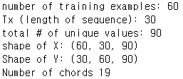
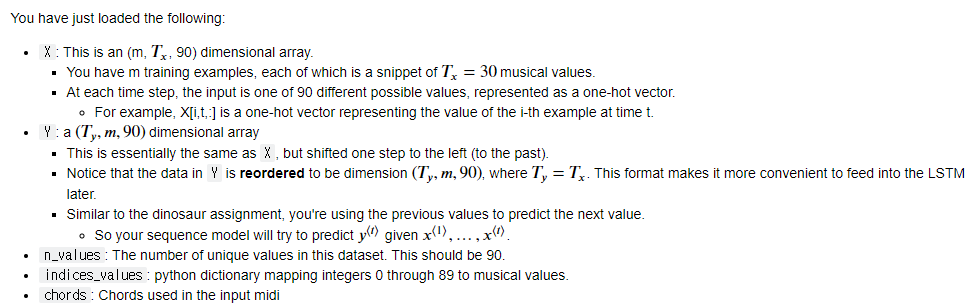
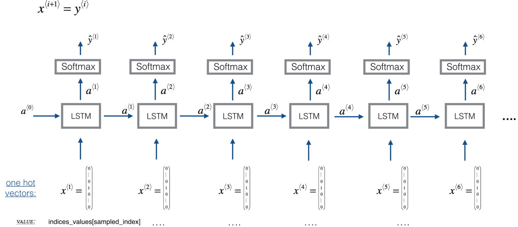
□ Model Overview
Here is the architecture of the model you'll use. It's similar to the Dinosaurus model, except that you'll implement it in Keras.
CHAPTER 3. 'Building the Model'
Now, you'll build and train a model that will learn musical patterns.
- The model takes input X of shape (𝑚,𝑇𝑥,90)(m,Tx,90) and labels Y of shape (𝑇𝑦,𝑚,90)(Ty,m,90).
- You'll use an LSTM with hidden states that have 𝑛𝑎=64na=64 dimensions.
# number of dimensions for the hidden state of each LSTM cell.
n_a = 64

n_values = 90 # number of music values
reshaper = Reshape((1, n_values))                  # Used in Step 2.B of djmodel(), below
LSTM_cell = LSTM(n_a, return_state = True)         # Used in Step 2.C
densor = Dense(n_values, activation='softmax')     # Used in Step 2.D
# UNQ_C1 (UNIQUE CELL IDENTIFIER, DO NOT EDIT)
# GRADED FUNCTION: djmodel

def djmodel(Tx, LSTM_cell, densor, reshaper):
    """
    Implement the djmodel composed of Tx LSTM cells where each cell is responsible
    for learning the following note based on the previous note and context.
    Each cell has the following schema:
            [X_{t}, a_{t-1}, c0_{t-1}] -> RESHAPE() -> LSTM() -> DENSE()
    Arguments:
        Tx -- length of the sequences in the corpus
        LSTM_cell -- LSTM layer instance
        densor -- Dense layer instance
        reshaper -- Reshape layer instance

    Returns:
        model -- a keras instance model with inputs [X, a0, c0]
    """
    # Get the shape of input values
    n_values = densor.units

    # Get the number of the hidden state vector
    n_a = LSTM_cell.units

    # Define the input layer and specify the shape
    X = Input(shape=(Tx, n_values))

    # Define the initial hidden state a0 and initial cell state c0
    # using `Input`
    a0 = Input(shape=(n_a,), name='a0')
    c0 = Input(shape=(n_a,), name='c0')
    a = a0
    c = c0
    ### START CODE HERE ###
    # Step 1: Create empty list to append the outputs while you iterate (≈1 line)
    outputs = []

    # Step 2: Loop over tx
    for t in range(Tx):

        # Step 2.A: select the "t"th time step vector from X.
        x = X[:, t, :]
        # Step 2.B: Use reshaper to reshape x to be (1, n_values) (≈1 line)
        x = reshaper(x)
        # Step 2.C: Perform one step of the LSTM_cell
        a, _, c = LSTM_cell(inputs=x, initial_state=[a, c])
        # Step 2.D: Apply densor to the hidden state output of LSTM_Cell
        out = densor(c)
        # Step 2.E: add the output to "outputs"
        outputs.append(out)

    # Step 3: Create model instance
    model = Model(inputs=[X, a0, c0], outputs=outputs)

    ### END CODE HERE ###

    return model
Create the model object
- Run the following cell to define your model.
- We will use Tx=30.
- This cell may take a few seconds to run.
model = djmodel(Tx=30, LSTM_cell=LSTM_cell, densor=densor, reshaper=reshaper)

# UNIT TEST
output = summary(model)
comparator(output, djmodel_out)

# Check your model
model.summary()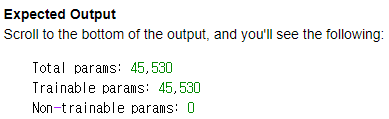
Compile the model for training
- You now need to compile your model to be trained.
- We will use:
- optimizer: Adam optimizer
- Loss function: categorical cross-entropy (for multi-class classification)
opt = Adam(lr=0.01, beta_1=0.9, beta_2=0.999, decay=0.01)

model.compile(optimizer=opt, loss='categorical_crossentropy', metrics=['accuracy'])
Finally, let's initialize a0 and c0 for the LSTM's initial state to be zero.
m = 60
a0 = np.zeros((m, n_a))
c0 = np.zeros((m, n_a))
Train the model
You're now ready to fit the model!
- You'll turn Y into a list, since the cost function expects Y to be provided in this format.
- list(Y) is a list with 30 items, where each of the list items is of shape (60,90).
- Train for 100 epochs (This will take a few minutes).
history = model.fit([X, a0, c0], list(Y), epochs=100, verbose = 0)

print(f"loss at epoch 1: {history.history['loss'][0]}")
print(f"loss at epoch 100: {history.history['loss'][99]}")
plt.plot(history.history['loss'])
CHAPTER 4. 'Generating Music'
□ Predicting & Sampling

At each step of sampling, you will:
- Take as input the activation 'a' and cell state 'c' from the previous state of the LSTM.
- Forward propagate by one step.
- Get a new output activation, as well as cell state.
- The new activation 'a' can then be used to generate the output using the fully connected layer, densor.
Initialization
- You'll initialize the following to be zeros:
- x0
- hidden state a0
- cell state c0
# UNQ_C2 (UNIQUE CELL IDENTIFIER, DO NOT EDIT)
# GRADED FUNCTION: music_inference_model

def music_inference_model(LSTM_cell, densor, Ty=100):
    """
    Uses the trained "LSTM_cell" and "densor" from model() to generate a sequence of values.

    Arguments:
    LSTM_cell -- the trained "LSTM_cell" from model(), Keras layer object
    densor -- the trained "densor" from model(), Keras layer object
    Ty -- integer, number of time steps to generate

    Returns:
    inference_model -- Keras model instance
    """

    # Get the shape of input values
    n_values = densor.units
    # Get the number of the hidden state vector
    n_a = LSTM_cell.units

    # Define the input of your model with a shape
    x0 = Input(shape=(1, n_values))


    # Define s0, initial hidden state for the decoder LSTM
    a0 = Input(shape=(n_a,), name='a0')
    c0 = Input(shape=(n_a,), name='c0')
    a = a0
    c = c0
    x = x0

    ### START CODE HERE ###
    # Step 1: Create an empty list of "outputs" to later store your predicted values (≈1 line)
    outputs = []

    # Step 2: Loop over Ty and generate a value at every time step
    for t in range(Ty):
        # Step 2.A: Perform one step of LSTM_cell. Use "x", not "x0" (≈1 line)
        a, _, c = LSTM_cell(x, initial_state = [a, c])

        # Step 2.B: Apply Dense layer to the hidden state output of the LSTM_cell (≈1 line)
        out = densor(a)
        # Step 2.C: Append the prediction "out" to "outputs". out.shape = (None, 90) (≈1 line)
        outputs.append(out)

        # Step 2.D:
        # Select the next value according to "out",
        # Set "x" to be the one-hot representation of the selected value
        # See instructions above.
        x = tf.math.argmax(out, 1)
        x = tf.one_hot(x, 90)
        # Step 2.E:
        # Use RepeatVector(1) to convert x into a tensor with shape=(None, 1, 90)
        x = RepeatVector(1)(x)

    # Step 3: Create model instance with the correct "inputs" and "outputs" (≈1 line)
    # choose the each initial values
    inference_model = Model(inputs=[x0, a0, c0], outputs=outputs)

    ### END CODE HERE ###

    return inference_model
Run the cell below to define your inference model. This model is hard coded to generate 50 values.
inference_model = music_inference_model(LSTM_cell, densor, Ty = 50)

# UNIT TEST
inference_summary = summary(inference_model)
comparator(inference_summary, music_inference_model_out)

# Check the inference model
inference_model.summary()
□ Initialize inference model
The following code creates the zero-valued vectors you will use to initialize x and the LSTM state variables a and c
x_initializer = np.zeros((1, 1, n_values))
a_initializer = np.zeros((1, n_a))
c_initializer = np.zeros((1, n_a))
# UNQ_C3 (UNIQUE CELL IDENTIFIER, DO NOT EDIT)
# GRADED FUNCTION: predict_and_sample

def predict_and_sample(inference_model, x_initializer = x_initializer, a_initializer = a_initializer,
                       c_initializer = c_initializer):
    """
    Predicts the next value of values using the inference model.

    Arguments:
    inference_model -- Keras model instance for inference time
    x_initializer -- numpy array of shape (1, 1, 90), one-hot vector initializing the values generation
    a_initializer -- numpy array of shape (1, n_a), initializing the hidden state of the LSTM_cell
    c_initializer -- numpy array of shape (1, n_a), initializing the cell state of the LSTM_cel

    Returns:
    results -- numpy-array of shape (Ty, 90), matrix of one-hot vectors representing the values generated
    indices -- numpy-array of shape (Ty, 1), matrix of indices representing the values generated
    """

    n_values = x_initializer.shape[2]

    ### START CODE HERE ###
    # Step 1: Use your inference model to predict an output sequence given x_initializer, a_initializer and c_initializer.
    pred = inference_model.predict([x_initializer, a_initializer, c_initializer])
    # Step 2: Convert "pred" into an np.array() of indices with the maximum probabilities
    indices = np.argmax(np.array(pred), axis = -1)
    # Step 3: Convert indices to one-hot vectors, the shape of the results should be (Ty, n_values)
    results = to_categorical(indices, num_classes=n_values)
    ### END CODE HERE ###

    return results, indices
results, indices = predict_and_sample(inference_model, x_initializer, a_initializer, c_initializer)

print("np.argmax(results[12]) =", np.argmax(results[12]))
print("np.argmax(results[17]) =", np.argmax(results[17]))
print("list(indices[12:18]) =", list(indices[12:18]))
□ Generate Music
Your RNN generates a sequence of values. The following code generates music by first calling your predict_and_sample() function. These values are then post-processed into musical chords (meaning that multiple values or notes can be played at the same time).
Most computational music algorithms use some post-processing because it's difficult to generate music that sounds good without it. The post-processing does things like clean up the generated audio by making sure the same sound is not repeated too many times, or that two successive notes are not too far from each other in pitch, and so on.
One could argue that a lot of these post-processing steps are hacks; also, a lot of the music generation literature has also focused on hand-crafting post-processors, and a lot of the output quality depends on the quality of the post-processing and not just the quality of the model. But this post-processing does make a huge difference, so you should use it in your implementation as well.
Let's make some music!
Run the following cell to generate music and record it into your out_stream. This can take a couple of minutes.
out_stream = generate_music(inference_model, indices_values, chords)

mid2wav('output/my_music.midi')
IPython.display.Audio('./output/rendered.wav')

IPython.display.Audio('./data/30s_trained_model.wav')
■ Congratulations!
You've completed this assignment, and generated your own jazz solo! The Coltranes would be proud.
By now, you've:
- Applied an LSTM to a music generation task
- Generated your own jazz music with deep learning
- Used the flexible Functional API to create a more complex model
This was a lengthy task. You should be proud of your hard work, and hopefully you have some good music to show for it. Cheers and see you next time!
What you should remember:
- A sequence model can be used to generate musical values, which are then post-processed into midi music.
- You can use a fairly similar model for tasks ranging from generating dinosaur names to generating original music, with the only major difference being the input fed to the model.
- In Keras, sequence generation involves defining layers with shared weights, which are then repeated for the different time steps 1,…,𝑇𝑥 .
■ 마무리
"Sequence Models" (Andrew Ng)의 1주차 "Improvise a Jazz Solo with an LSTM Network"의 실습에 대해서 정리해봤습니다.
그럼 오늘 하루도 즐거운 나날 되길 기도하겠습니다
좋아요와 댓글 부탁드립니다 :)
감사합니다.
'COURSERA' 카테고리의 다른 글
| week 2_Natural Language Processing & Word Embeddings 연습 문제 (Andrew Ng) (0) | 2022.04.27 |
|---|---|
| week 2_NLP and Word Embeddings (Andrew Ng) (0) | 2022.04.27 |
| week 1_Character level language model - Dinosaurus Island 실습 (Andrew Ng) (0) | 2022.04.27 |
| week 1_Building your Recurrent Neural Network - Step by Step 실습 (Andrew Ng) (0) | 2022.04.27 |
| week 1_Recurrent Neural Networks 연습 문제 (Andrew Ng) (0) | 2022.04.27 |


댓글