
안녕하세요, HELLO
오늘은 DeepLearning.AI에서 진행하는 앤드류 응(Andrew Ng) 교수님의 딥러닝 전문화의 마지막이며, 다섯 번째 과정인 "Sequence Models"을 정리하려고 합니다.
"Sequence Models"의 강의를 통해 '시퀀스 모델과 음성 인식, 음악 합성, 챗봇, 기계 번역, 자연어 처리(NLP)' 등을 이해하고, 순환 신경망(RNN)과 GRU 및 LSTM, 트랜스포머 모델에 대해서 배우게 됩니다. 강의는 아래와 같이 구성되어 있습니다.
~ Recurrent Neural Networks
~ Natural Language Processing & Word Embeddings
~ Sequence Models & Attention Mechanism
~ Transformer Network
"Sequence Models" (Andrew Ng)의 1주차 "Building your Recurrent Neural Network - Step by Step"의 실습 내용입니다.
By the end of this assignment, you'll be able to:
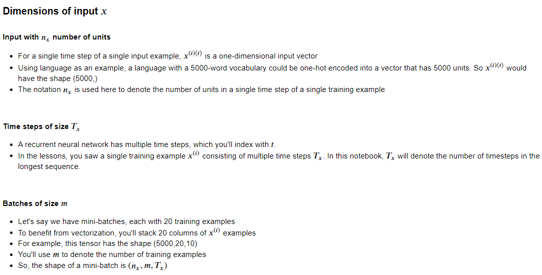
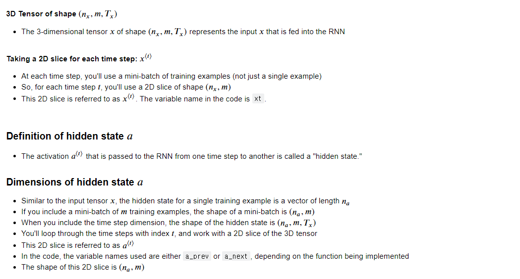
- Define notation for building sequence models
- Describe the architecture of a basic RNN
- Identify the main components of an LSTM
- Implement backpropagation through time for a basic RNN and an LSTM
- Give examples of several types of RNN
CHAPTER 1. 'Packages'
CHAPTER 2. 'Forward Propagation for the Basic Recurrent Neural Network'
CHAPTER 3. 'Long Short-Term Memory (LSTM) Network'
CHAPTER 4. 'Backpropagation in Recurrent Neural Networks (OPTIONAL / UNGRADED)'
CHAPTER 1. 'Packages'
import numpy as np
from rnn_utils import *
from public_tests import *
CHAPTER 2. 'Forward Propagation for the Basic Recurrent Neural Network'

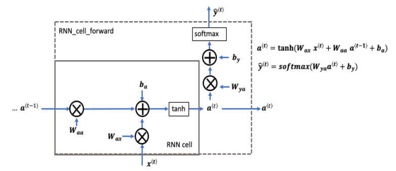
Here's how you can implement an RNN:
Steps:
- Implement the calculations needed for one time step of the RNN.
- Implement a loop over 𝑇𝑥Tx time steps in order to process all the inputs, one at a time.
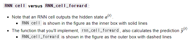
□ RNN Cell
You can think of the recurrent neural network as the repeated use of a single cell. First, you'll implement the computations for a single time step. The following figure describes the operations for a single time step of an RNN cell:
# UNQ_C1 (UNIQUE CELL IDENTIFIER, DO NOT EDIT)
# GRADED FUNCTION: rnn_cell_forward

def rnn_cell_forward(xt, a_prev, parameters):
    """
    Implements a single forward step of the RNN-cell as described in Figure (2)

    Arguments:
    xt -- your input data at timestep "t", numpy array of shape (n_x, m).
    a_prev -- Hidden state at timestep "t-1", numpy array of shape (n_a, m)
    parameters -- python dictionary containing:
                        Wax -- Weight matrix multiplying the input, numpy array of shape (n_a, n_x)
                        Waa -- Weight matrix multiplying the hidden state, numpy array of shape (n_a, n_a)
                        Wya -- Weight matrix relating the hidden-state to the output, numpy array of shape (n_y, n_a)
                        ba --  Bias, numpy array of shape (n_a, 1)
                        by -- Bias relating the hidden-state to the output, numpy array of shape (n_y, 1)
    Returns:
    a_next -- next hidden state, of shape (n_a, m)
    yt_pred -- prediction at timestep "t", numpy array of shape (n_y, m)
    cache -- tuple of values needed for the backward pass, contains (a_next, a_prev, xt, parameters)
    """

    # Retrieve parameters from "parameters"
    Wax = parameters["Wax"]
    Waa = parameters["Waa"]
    Wya = parameters["Wya"]
    ba = parameters["ba"]
    by = parameters["by"]

    ### START CODE HERE ### (≈2 lines)
    # compute next activation state using the formula given above
    a_next = np.tanh(np.dot(Wax, xt) + np.dot(Waa, a_prev) + ba)
    # compute output of the current cell using the formula given above
    yt_pred = softmax(np.dot(Wya, a_next) + by)
    ### END CODE HERE ###

    # store values you need for backward propagation in cache
    cache = (a_next, a_prev, xt, parameters)

    return a_next, yt_pred, cache
np.random.seed(1)
xt_tmp = np.random.randn(3, 10)
a_prev_tmp = np.random.randn(5, 10)
parameters_tmp = {}
parameters_tmp['Waa'] = np.random.randn(5, 5)
parameters_tmp['Wax'] = np.random.randn(5, 3)
parameters_tmp['Wya'] = np.random.randn(2, 5)
parameters_tmp['ba'] = np.random.randn(5, 1)
parameters_tmp['by'] = np.random.randn(2, 1)

a_next_tmp, yt_pred_tmp, cache_tmp = rnn_cell_forward(xt_tmp, a_prev_tmp, parameters_tmp)
print("a_next[4] = \n", a_next_tmp[4])
print("a_next.shape = \n", a_next_tmp.shape)
print("yt_pred[1] =\n", yt_pred_tmp[1])
print("yt_pred.shape = \n", yt_pred_tmp.shape)

# UNIT TESTS
rnn_cell_forward_tests(rnn_cell_forward)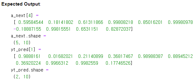
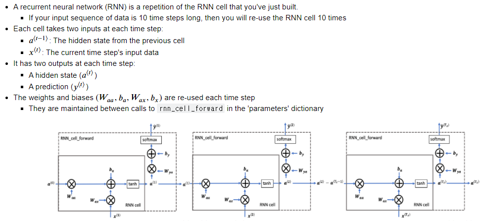
□ RNN Forward Pass
# UNQ_C2 (UNIQUE CELL IDENTIFIER, DO NOT EDIT)
# GRADED FUNCTION: rnn_forward

def rnn_forward(x, a0, parameters):
    """
    Implement the forward propagation of the recurrent neural network described in Figure (3).

    Arguments:
    x -- Input data for every time-step, of shape (n_x, m, T_x).
    a0 -- Initial hidden state, of shape (n_a, m)
    parameters -- python dictionary containing:
                        Waa -- Weight matrix multiplying the hidden state, numpy array of shape (n_a, n_a)
                        Wax -- Weight matrix multiplying the input, numpy array of shape (n_a, n_x)
                        Wya -- Weight matrix relating the hidden-state to the output, numpy array of shape (n_y, n_a)
                        ba --  Bias numpy array of shape (n_a, 1)
                        by -- Bias relating the hidden-state to the output, numpy array of shape (n_y, 1)

    Returns:
    a -- Hidden states for every time-step, numpy array of shape (n_a, m, T_x)
    y_pred -- Predictions for every time-step, numpy array of shape (n_y, m, T_x)
    caches -- tuple of values needed for the backward pass, contains (list of caches, x)
    """

    # Initialize "caches" which will contain the list of all caches
    caches = []

    # Retrieve dimensions from shapes of x and parameters["Wya"]
    n_x, m, T_x = x.shape
    n_y, n_a = parameters["Wya"].shape

    ### START CODE HERE ###

    # initialize "a" and "y_pred" with zeros (≈2 lines)
    a = np.zeros((n_a, m, T_x))
    y_pred = np.zeros((n_y, m, T_x))

    # Initialize a_next (≈1 line)
    a_next = a0

    # loop over all time-steps
    for t in range(T_x):
        # Update next hidden state, compute the prediction, get the cache (≈1 line)
        a_next, yt_pred, cache = rnn_cell_forward(x[:,:,t] ,a_next, parameters)
        # Save the value of the new "next" hidden state in a (≈1 line)
        a[:,:,t] = a_next
        # Save the value of the prediction in y (≈1 line)
        y_pred[:,:,t] = yt_pred
        # Append "cache" to "caches" (≈1 line)
        caches.append(cache)
    ### END CODE HERE ###

    # store values needed for backward propagation in cache
    caches = (caches, x)

    return a, y_pred, caches
np.random.seed(1)
x_tmp = np.random.randn(3, 10, 4)
a0_tmp = np.random.randn(5, 10)
parameters_tmp = {}
parameters_tmp['Waa'] = np.random.randn(5, 5)
parameters_tmp['Wax'] = np.random.randn(5, 3)
parameters_tmp['Wya'] = np.random.randn(2, 5)
parameters_tmp['ba'] = np.random.randn(5, 1)
parameters_tmp['by'] = np.random.randn(2, 1)

a_tmp, y_pred_tmp, caches_tmp = rnn_forward(x_tmp, a0_tmp, parameters_tmp)
print("a[4][1] = \n", a_tmp[4][1])
print("a.shape = \n", a_tmp.shape)
print("y_pred[1][3] =\n", y_pred_tmp[1][3])
print("y_pred.shape = \n", y_pred_tmp.shape)
print("caches[1][1][3] =\n", caches_tmp[1][1][3])
print("len(caches) = \n", len(caches_tmp))

#UNIT TEST
rnn_forward_test(rnn_forward)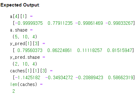
CHAPTER 3. 'Long Short-Term Memory (LSTM) Network'
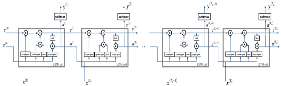
The following figure shows the operations of an LSTM cell:
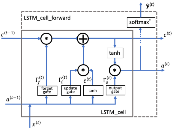
□ Overview of gates and states
# UNQ_C3 (UNIQUE CELL IDENTIFIER, DO NOT EDIT)
# GRADED FUNCTION: lstm_cell_forward
def lstm_cell_forward(xt, a_prev, c_prev, parameters):
"""
Implement a single forward step of the LSTM-cell as described in Figure (4)
Arguments:
xt -- your input data at timestep "t", numpy array of shape (n_x, m).
a_prev -- Hidden state at timestep "t-1", numpy array of shape (n_a, m)
c_prev -- Memory state at timestep "t-1", numpy array of shape (n_a, m)
parameters -- python dictionary containing:
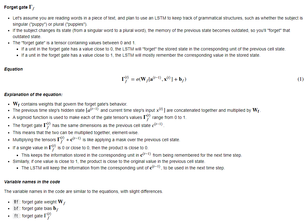
Wf -- Weight matrix of the forget gate, numpy array of shape (n_a, n_a + n_x)
bf -- Bias of the forget gate, numpy array of shape (n_a, 1)
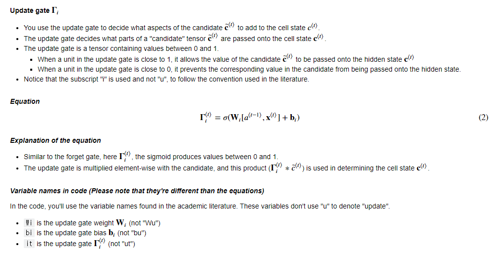
Wi -- Weight matrix of the update gate, numpy array of shape (n_a, n_a + n_x)
bi -- Bias of the update gate, numpy array of shape (n_a, 1)
Wc -- Weight matrix of the first "tanh", numpy array of shape (n_a, n_a + n_x)
bc -- Bias of the first "tanh", numpy array of shape (n_a, 1)
Wo -- Weight matrix of the output gate, numpy array of shape (n_a, n_a + n_x)
bo -- Bias of the output gate, numpy array of shape (n_a, 1)
Wy -- Weight matrix relating the hidden-state to the output, numpy array of shape (n_y, n_a)
by -- Bias relating the hidden-state to the output, numpy array of shape (n_y, 1)
Returns:
a_next -- next hidden state, of shape (n_a, m)
c_next -- next memory state, of shape (n_a, m)
yt_pred -- prediction at timestep "t", numpy array of shape (n_y, m)
cache -- tuple of values needed for the backward pass, contains (a_next, c_next, a_prev, c_prev, xt, parameters)
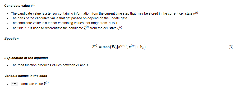
Note: ft/it/ot stand for the forget/update/output gates, cct stands for the candidate value (c tilde),
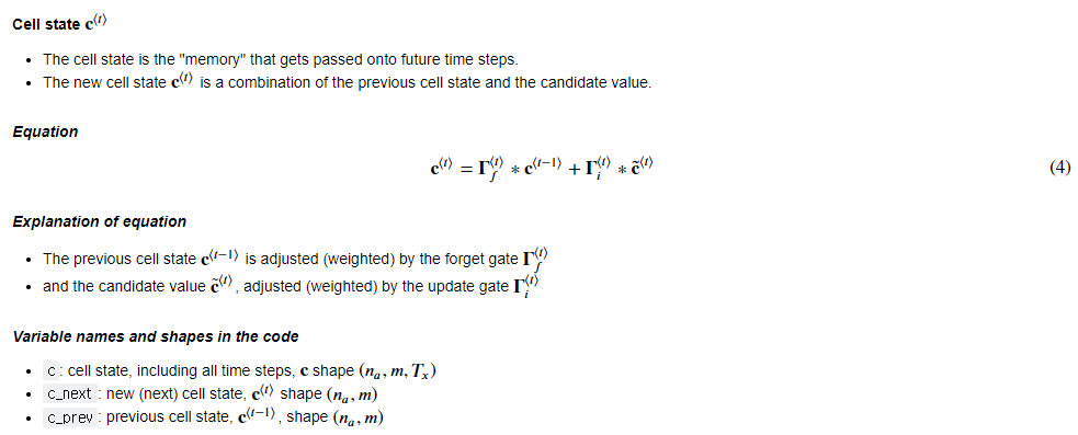
c stands for the cell state (memory)
"""
# Retrieve parameters from "parameters"
Wf = parameters["Wf"] # forget gate weight
bf = parameters["bf"]
Wi = parameters["Wi"] # update gate weight (notice the variable name)
bi = parameters["bi"] # (notice the variable name)
Wc = parameters["Wc"] # candidate value weight
bc = parameters["bc"]
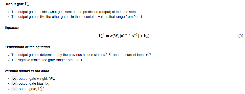
Wo = parameters["Wo"] # output gate weight
bo = parameters["bo"]
Wy = parameters["Wy"] # prediction weight
by = parameters["by"]
# Retrieve dimensions from shapes of xt and Wy
n_x, m = xt.shape
n_y, n_a = Wy.shape
### START CODE HERE ###
# Concatenate a_prev and xt (≈1 line)
concat = np.concatenate((a_prev, xt), axis=0)
# Compute values for ft, it, cct, c_next, ot, a_next using the formulas given figure (4) (≈6 lines)
ft = sigmoid(np.dot(Wf, concat) + bf)
it = sigmoid(np.dot(Wi, concat) + bi)
cct = np.tanh(np.dot(Wc, concat) + bc)
c_next = ft * c_prev + it * cct
ot = sigmoid(np.dot(Wo, concat) + bo)
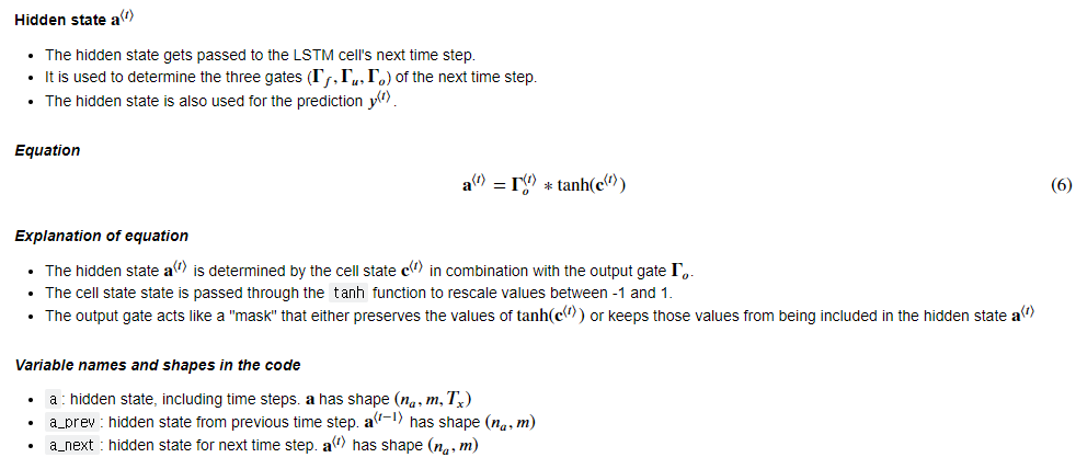
a_next = ot * np.tanh(c_next)
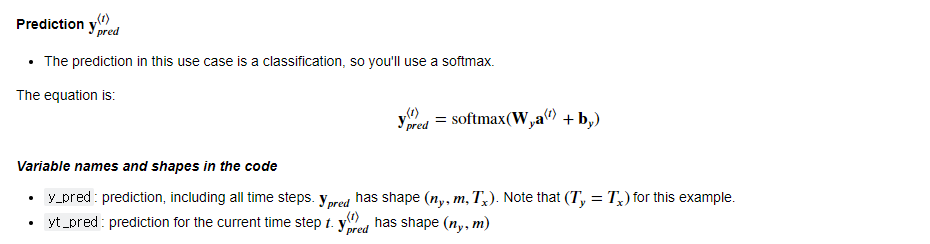
# Compute prediction of the LSTM cell (≈1 line)
yt_pred = softmax(np.dot(Wy, a_next) + by)
### END CODE HERE ###
# store values needed for backward propagation in cache
cache = (a_next, c_next, a_prev, c_prev, ft, it, cct, ot, xt, parameters)
return a_next, c_next, yt_pred, cache
np.random.seed(1)
xt_tmp = np.random.randn(3, 10)
a_prev_tmp = np.random.randn(5, 10)
c_prev_tmp = np.random.randn(5, 10)
parameters_tmp = {}
parameters_tmp['Wf'] = np.random.randn(5, 5 + 3)
parameters_tmp['bf'] = np.random.randn(5, 1)
parameters_tmp['Wi'] = np.random.randn(5, 5 + 3)
parameters_tmp['bi'] = np.random.randn(5, 1)
parameters_tmp['Wo'] = np.random.randn(5, 5 + 3)
parameters_tmp['bo'] = np.random.randn(5, 1)
parameters_tmp['Wc'] = np.random.randn(5, 5 + 3)
parameters_tmp['bc'] = np.random.randn(5, 1)
parameters_tmp['Wy'] = np.random.randn(2, 5)
parameters_tmp['by'] = np.random.randn(2, 1)

a_next_tmp, c_next_tmp, yt_tmp, cache_tmp = lstm_cell_forward(xt_tmp, a_prev_tmp, c_prev_tmp, parameters_tmp)

print("a_next[4] = \n", a_next_tmp[4])
print("a_next.shape = ", a_next_tmp.shape)
print("c_next[2] = \n", c_next_tmp[2])
print("c_next.shape = ", c_next_tmp.shape)
print("yt[1] =", yt_tmp[1])
print("yt.shape = ", yt_tmp.shape)
print("cache[1][3] =\n", cache_tmp[1][3])
print("len(cache) = ", len(cache_tmp))

# UNIT TEST
lstm_cell_forward_test(lstm_cell_forward)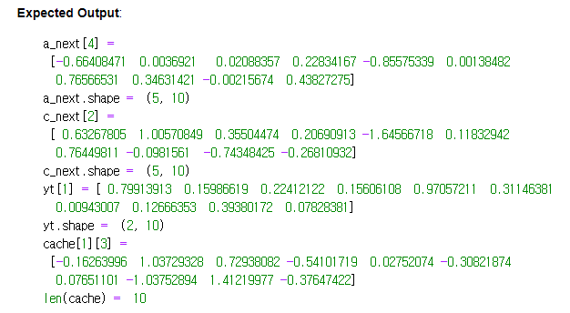
■ Forward Pass for LSTM
Now that you have implemented one step of an LSTM, you can iterate this over it using a for loop to process a sequence of 𝑇𝑥 inputs.
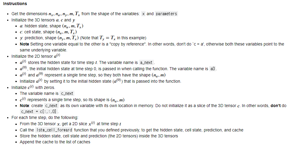
# UNQ_C4 (UNIQUE CELL IDENTIFIER, DO NOT EDIT)
# GRADED FUNCTION: lstm_forward

def lstm_forward(x, a0, parameters):
    """
    Implement the forward propagation of the recurrent neural network using an LSTM-cell described in Figure (4).

    Arguments:
    x -- Input data for every time-step, of shape (n_x, m, T_x).
    a0 -- Initial hidden state, of shape (n_a, m)
    parameters -- python dictionary containing:
                        Wf -- Weight matrix of the forget gate, numpy array of shape (n_a, n_a + n_x)
                        bf -- Bias of the forget gate, numpy array of shape (n_a, 1)
                        Wi -- Weight matrix of the update gate, numpy array of shape (n_a, n_a + n_x)
                        bi -- Bias of the update gate, numpy array of shape (n_a, 1)
                        Wc -- Weight matrix of the first "tanh", numpy array of shape (n_a, n_a + n_x)
                        bc -- Bias of the first "tanh", numpy array of shape (n_a, 1)
                        Wo -- Weight matrix of the output gate, numpy array of shape (n_a, n_a + n_x)
                        bo -- Bias of the output gate, numpy array of shape (n_a, 1)
                        Wy -- Weight matrix relating the hidden-state to the output, numpy array of shape (n_y, n_a)
                        by -- Bias relating the hidden-state to the output, numpy array of shape (n_y, 1)

    Returns:
    a -- Hidden states for every time-step, numpy array of shape (n_a, m, T_x)
    y -- Predictions for every time-step, numpy array of shape (n_y, m, T_x)
    c -- The value of the cell state, numpy array of shape (n_a, m, T_x)
    caches -- tuple of values needed for the backward pass, contains (list of all the caches, x)
    """

    # Initialize "caches", which will track the list of all the caches
    caches = []

    ### START CODE HERE ###
    Wy = parameters['Wy'] # saving parameters['Wy'] in a local variable in case students use Wy instead of parameters['Wy']
    # Retrieve dimensions from shapes of x and parameters['Wy'] (≈2 lines)
    n_x, m, T_x = x.shape
    n_y, n_a = Wy.shape

    # initialize "a", "c" and "y" with zeros (≈3 lines)
    a = np.zeros((n_a, m, T_x))
    c = np.zeros((n_a, m, T_x))
    y = np.zeros((n_y, m, T_x))

    # Initialize a_next and c_next (≈2 lines)
    a_next = a0
    c_next = np.zeros((n_a, m))

    # loop over all time-steps
    for t in range(T_x):
        # Get the 2D slice 'xt' from the 3D input 'x' at time step 't'
        xt = x[:,:,t]
        # Update next hidden state, next memory state, compute the prediction, get the cache (≈1 line)
        a_next, c_next, yt, cache = lstm_cell_forward(xt, a_next, c_next, parameters)
        # Save the value of the new "next" hidden state in a (≈1 line)
        a[:,:,t] = a_next
        # Save the value of the next cell state (≈1 line)
        c[:,:,t]  = c_next
        # Save the value of the prediction in y (≈1 line)
        y[:,:,t] = yt
        # Append the cache into caches (≈1 line)
        caches.append(cache)

    ### END CODE HERE ###

    # store values needed for backward propagation in cache
    caches = (caches, x)

    return a, y, c, caches
np.random.seed(1)
x_tmp = np.random.randn(3, 10, 7)
a0_tmp = np.random.randn(5, 10)
parameters_tmp = {}
parameters_tmp['Wf'] = np.random.randn(5, 5 + 3)
parameters_tmp['bf'] = np.random.randn(5, 1)
parameters_tmp['Wi'] = np.random.randn(5, 5 + 3)
parameters_tmp['bi']= np.random.randn(5, 1)
parameters_tmp['Wo'] = np.random.randn(5, 5 + 3)
parameters_tmp['bo'] = np.random.randn(5, 1)
parameters_tmp['Wc'] = np.random.randn(5, 5 + 3)
parameters_tmp['bc'] = np.random.randn(5, 1)
parameters_tmp['Wy'] = np.random.randn(2, 5)
parameters_tmp['by'] = np.random.randn(2, 1)

a_tmp, y_tmp, c_tmp, caches_tmp = lstm_forward(x_tmp, a0_tmp, parameters_tmp)
print("a[4][3][6] = ", a_tmp[4][3][6])
print("a.shape = ", a_tmp.shape)
print("y[1][4][3] =", y_tmp[1][4][3])
print("y.shape = ", y_tmp.shape)
print("caches[1][1][1] =\n", caches_tmp[1][1][1])
print("c[1][2][1]", c_tmp[1][2][1])
print("len(caches) = ", len(caches_tmp))

# UNIT TEST
lstm_forward_test(lstm_forward)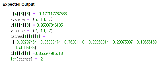
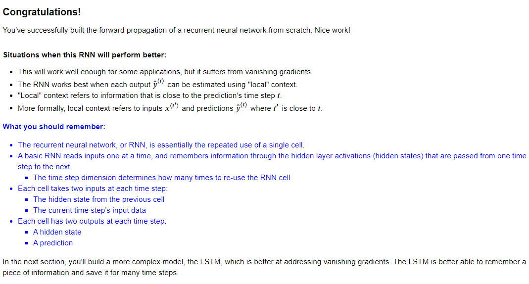
Congratulations!
You have now implemented the forward passes for both the basic RNN and the LSTM. When using a deep learning framework, implementing the forward pass is sufficient to build systems that achieve great performance. The framework will take care of the rest.
What you should remember:
Let's recap all you've accomplished so far. You have:
- Used notation for building sequence models
- Become familiar with the architecture of a basic RNN and an LSTM, and can describe their components
The rest of this notebook is optional, and will not be graded, but as always, you are encouraged to push your own understanding! Good luck and have fun.
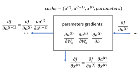
CHAPTER 4. 'Backpropagation in Recurrent Neural Networks (OPTIONAL / UNGRADED)'
In modern deep learning frameworks, you only have to implement the forward pass, and the framework takes care of the backward pass, so most deep learning engineers do not need to bother with the details of the backward pass. If, however, you are an expert in calculus (or are just curious) and want to see the details of backprop in RNNs, you can work through this optional portion of the notebook.
When in an earlier course you implemented a simple (fully connected) neural network, you used backpropagation to compute the derivatives with respect to the cost to update the parameters. Similarly, in recurrent neural networks you can calculate the derivatives with respect to the cost in order to update the parameters. The backprop equations are quite complicated, and so were not derived in lecture. However, they're briefly presented for your viewing pleasure below.
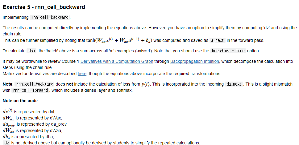
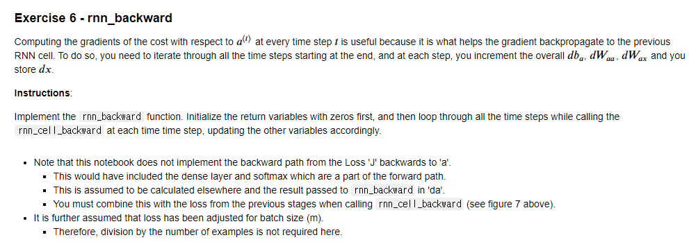
Note that this notebook does not implement the backward path from the Loss 'J' backwards to 'a'. This would have included the dense layer and softmax, which are a part of the forward path. This is assumed to be calculated elsewhere and the result passed to rnn_backward in 'da'. It is further assumed that loss has been adjusted for batch size (m) and division by the number of examples is not required here.
This section is optional and ungraded, because it's more difficult and has fewer details regarding its implementation. Note that this section only implements key elements of the full path.
□ Basic RNN Backward Pass
Begin by computing the backward pass for the basic RNN cell. Then, in the following sections, iterate through the cells.
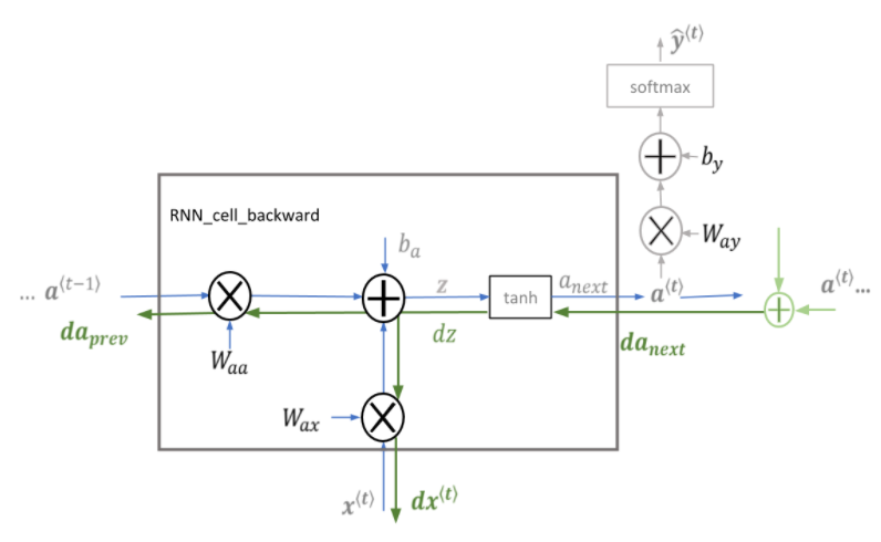
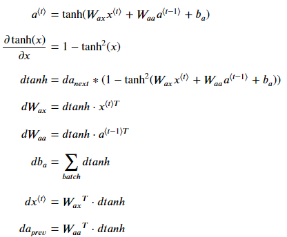
■ Equations
To compute rnn_cell_backward, you can use the following equations. It's a good exercise to derive them by hand. Here, ∗ denotes element-wise multiplication while the absence of a symbol indicates matrix multiplication.
# UNGRADED FUNCTION: rnn_cell_backward

def rnn_cell_backward(da_next, cache):
    """
    Implements the backward pass for the RNN-cell (single time-step).

    Arguments:
    da_next -- Gradient of loss with respect to next hidden state
    cache -- python dictionary containing useful values (output of rnn_cell_forward())

    Returns:
    gradients -- python dictionary containing:
                        dx -- Gradients of input data, of shape (n_x, m)
                        da_prev -- Gradients of previous hidden state, of shape (n_a, m)
                        dWax -- Gradients of input-to-hidden weights, of shape (n_a, n_x)
                        dWaa -- Gradients of hidden-to-hidden weights, of shape (n_a, n_a)
                        dba -- Gradients of bias vector, of shape (n_a, 1)
    """

    # Retrieve values from cache
    (a_next, a_prev, xt, parameters) = cache

    # Retrieve values from parameters
    Wax = parameters["Wax"]
    Waa = parameters["Waa"]
    Wya = parameters["Wya"]
    ba = parameters["ba"]
    by = parameters["by"]

    ### START CODE HERE ###
    # compute the gradient of dtanh term using a_next and da_next (≈1 line)
    dtanh = da_next * (1- a_next **2)

    # compute the gradient of the loss with respect to Wax (≈2 lines)
    dxt = np.dot(Wax.T, dtanh)
    dWax = np.dot(dtanh, xt.T)

    # compute the gradient with respect to Waa (≈2 lines)
    da_prev = np.dot(Waa.T, dtanh)
    dWaa = np.dot(dtanh, a_prev.T)

    # compute the gradient with respect to b (≈1 line)
    dba = np.sum(dtanh, axis=1, keepdims = True)

    ### END CODE HERE ###

    # Store the gradients in a python dictionary
    gradients = {"dxt": dxt, "da_prev": da_prev, "dWax": dWax, "dWaa": dWaa, "dba": dba}

    return gradients
np.random.seed(1)
xt_tmp = np.random.randn(3,10)
a_prev_tmp = np.random.randn(5,10)
parameters_tmp = {}
parameters_tmp['Wax'] = np.random.randn(5,3)
parameters_tmp['Waa'] = np.random.randn(5,5)
parameters_tmp['Wya'] = np.random.randn(2,5)
parameters_tmp['ba'] = np.random.randn(5,1)
parameters_tmp['by'] = np.random.randn(2,1)

a_next_tmp, yt_tmp, cache_tmp = rnn_cell_forward(xt_tmp, a_prev_tmp, parameters_tmp)

da_next_tmp = np.random.randn(5,10)
gradients_tmp = rnn_cell_backward(da_next_tmp, cache_tmp)
print("gradients[\"dxt\"][1][2] =", gradients_tmp["dxt"][1][2])
print("gradients[\"dxt\"].shape =", gradients_tmp["dxt"].shape)
print("gradients[\"da_prev\"][2][3] =", gradients_tmp["da_prev"][2][3])
print("gradients[\"da_prev\"].shape =", gradients_tmp["da_prev"].shape)
print("gradients[\"dWax\"][3][1] =", gradients_tmp["dWax"][3][1])
print("gradients[\"dWax\"].shape =", gradients_tmp["dWax"].shape)
print("gradients[\"dWaa\"][1][2] =", gradients_tmp["dWaa"][1][2])
print("gradients[\"dWaa\"].shape =", gradients_tmp["dWaa"].shape)
print("gradients[\"dba\"][4] =", gradients_tmp["dba"][4])
print("gradients[\"dba\"].shape =", gradients_tmp["dba"].shape)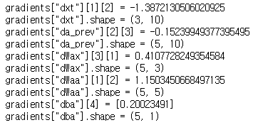
# UNGRADED FUNCTION: rnn_backward

def rnn_backward(da, caches):
    """
    Implement the backward pass for a RNN over an entire sequence of input data.

    Arguments:
    da -- Upstream gradients of all hidden states, of shape (n_a, m, T_x)
    caches -- tuple containing information from the forward pass (rnn_forward)

    Returns:
    gradients -- python dictionary containing:
                        dx -- Gradient w.r.t. the input data, numpy-array of shape (n_x, m, T_x)
                        da0 -- Gradient w.r.t the initial hidden state, numpy-array of shape (n_a, m)
                        dWax -- Gradient w.r.t the input's weight matrix, numpy-array of shape (n_a, n_x)
                        dWaa -- Gradient w.r.t the hidden state's weight matrix, numpy-arrayof shape (n_a, n_a)
                        dba -- Gradient w.r.t the bias, of shape (n_a, 1)
    """

    ### START CODE HERE ###

    # Retrieve values from the first cache (t=1) of caches (≈2 lines)
    (caches, x) = caches
    (a1, a0, x1, parameters) = caches[0]

    # Retrieve dimensions from da's and x1's shapes (≈2 lines)
    n_a, m, T_x = da.shape
    n_x, m = x1.shape

    # initialize the gradients with the right sizes (≈6 lines)
    dx = np.zeros((n_x, m, T_x))
    dWax = np.zeros((n_a, n_x))
    dWaa = np.zeros((n_a, n_a))
    dba = np.zeros((n_a, 1))
    da0 = np.zeros((n_a, m))
    da_prevt = np.zeros((n_a, m))

    # Loop through all the time steps
    for t in reversed(range(T_x)):
        # Compute gradients at time step t. Choose wisely the "da_next" and the "cache" to use in the backward propagation step. (≈1 line)
        gradients = rnn_cell_backward(da[:,:,t], caches[t])
        # Retrieve derivatives from gradients (≈ 1 line)
        dxt, da_prevt, dWaxt, dWaat, dbat = gradients["dxt"], gradients["da_prev"], gradients["dWax"], gradients["dWaa"], gradients["dba"]
        # Increment global derivatives w.r.t parameters by adding their derivative at time-step t (≈4 lines)
        dx[:, :, t] = dxt
        dWax += dWaxt
        dWaa += dWaat
        dba += dbat

    # Set da0 to the gradient of a which has been backpropagated through all time-steps (≈1 line)
    da0 = da_prevt
    ### END CODE HERE ###

    # Store the gradients in a python dictionary
    gradients = {"dx": dx, "da0": da0, "dWax": dWax, "dWaa": dWaa,"dba": dba}

    return gradients
np.random.seed(1)
x_tmp = np.random.randn(3,10,4)
a0_tmp = np.random.randn(5,10)
parameters_tmp = {}
parameters_tmp['Wax'] = np.random.randn(5,3)
parameters_tmp['Waa'] = np.random.randn(5,5)
parameters_tmp['Wya'] = np.random.randn(2,5)
parameters_tmp['ba'] = np.random.randn(5,1)
parameters_tmp['by'] = np.random.randn(2,1)

a_tmp, y_tmp, caches_tmp = rnn_forward(x_tmp, a0_tmp, parameters_tmp)
da_tmp = np.random.randn(5, 10, 4)
gradients_tmp = rnn_backward(da_tmp, caches_tmp)

print("gradients[\"dx\"][1][2] =", gradients_tmp["dx"][1][2])
print("gradients[\"dx\"].shape =", gradients_tmp["dx"].shape)
print("gradients[\"da0\"][2][3] =", gradients_tmp["da0"][2][3])
print("gradients[\"da0\"].shape =", gradients_tmp["da0"].shape)
print("gradients[\"dWax\"][3][1] =", gradients_tmp["dWax"][3][1])
print("gradients[\"dWax\"].shape =", gradients_tmp["dWax"].shape)
print("gradients[\"dWaa\"][1][2] =", gradients_tmp["dWaa"][1][2])
print("gradients[\"dWaa\"].shape =", gradients_tmp["dWaa"].shape)
print("gradients[\"dba\"][4] =", gradients_tmp["dba"][4])
print("gradients[\"dba\"].shape =", gradients_tmp["dba"].shape)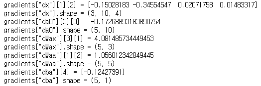
□ LSTM Backward Pass
■ One Step Backward
The LSTM backward pass is slightly more complicated than the forward pass.
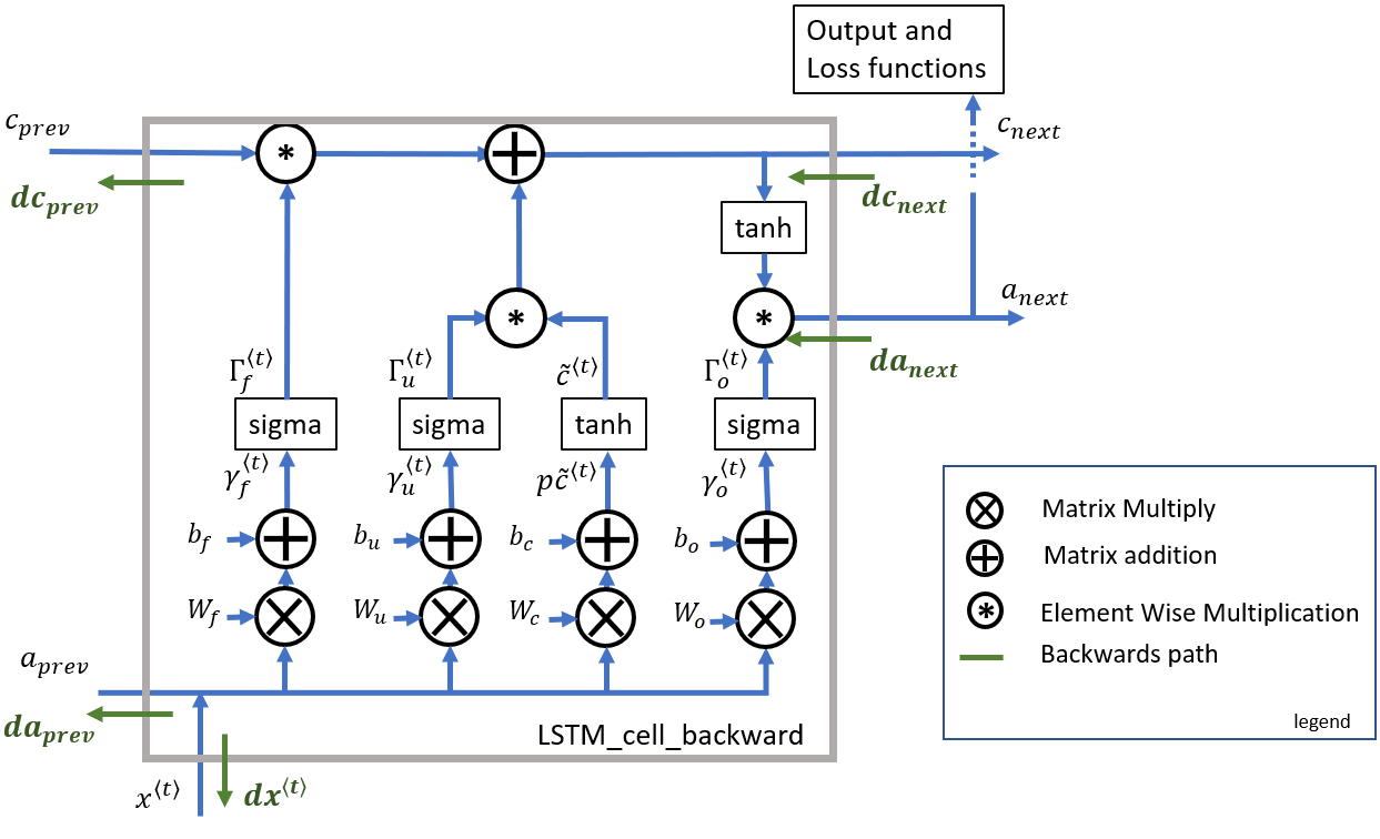
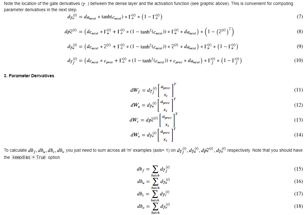
■ Gate Derivatives
# UNGRADED FUNCTION: lstm_cell_backward
def lstm_cell_backward(da_next, dc_next, cache):
"""
Implement the backward pass for the LSTM-cell (single time-step).
Arguments:
da_next -- Gradients of next hidden state, of shape (n_a, m)
dc_next -- Gradients of next cell state, of shape (n_a, m)
cache -- cache storing information from the forward pass
Returns:
gradients -- python dictionary containing:
dxt -- Gradient of input data at time-step t, of shape (n_x, m)
da_prev -- Gradient w.r.t. the previous hidden state, numpy array of shape (n_a, m)
dc_prev -- Gradient w.r.t. the previous memory state, of shape (n_a, m, T_x)
dWf -- Gradient w.r.t. the weight matrix of the forget gate, numpy array of shape (n_a, n_a + n_x)
dWi -- Gradient w.r.t. the weight matrix of the update gate, numpy array of shape (n_a, n_a + n_x)
dWc -- Gradient w.r.t. the weight matrix of the memory gate, numpy array of shape (n_a, n_a + n_x)
dWo -- Gradient w.r.t. the weight matrix of the output gate, numpy array of shape (n_a, n_a + n_x)
dbf -- Gradient w.r.t. biases of the forget gate, of shape (n_a, 1)
dbi -- Gradient w.r.t. biases of the update gate, of shape (n_a, 1)
dbc -- Gradient w.r.t. biases of the memory gate, of shape (n_a, 1)
dbo -- Gradient w.r.t. biases of the output gate, of shape (n_a, 1)
"""
# Retrieve information from "cache"
(a_next, c_next, a_prev, c_prev, ft, it, cct, ot, xt, parameters) = cache
### START CODE HERE ###
# Retrieve dimensions from xt's and a_next's shape (≈2 lines)
n_x, m = xt.shape
n_a, m = a_next.shape
# Compute gates related derivatives. Their values can be found by looking carefully at equations (7) to (10) (≈4 lines)
dot = da_next * np.tanh(c_next) * ot * (1 - ot)
dcct = (dc_next * it + ot * (1 - np.square(np.tanh(c_next))) * it * da_next) * (1 - np.square(cct))
dit = (dc_next * cct + ot * (1 - np.square(np.tanh(c_next))) * cct * da_next) * it * (1 - it)
dft = (dc_next * c_prev + ot *(1 - np.square(np.tanh(c_next))) * c_prev * da_next) * ft * (1 - ft)
# Compute parameters related derivatives. Use equations (11)-(18) (≈8 lines)
concat = np.concatenate((a_prev, xt), axis=0)
dWf = np.dot(dft, concat.T)
dWi = np.dot(dit, concat.T)
dWc = np.dot(dcct, concat.T)
dWo = np.dot(dot, concat.T)
dbf = np.sum(dft, axis=1 ,keepdims = True)
dbi = np.sum(dit, axis=1, keepdims = True)
dbc = np.sum(dcct, axis=1, keepdims = True)
dbo = np.sum(dot, axis=1, keepdims = True)
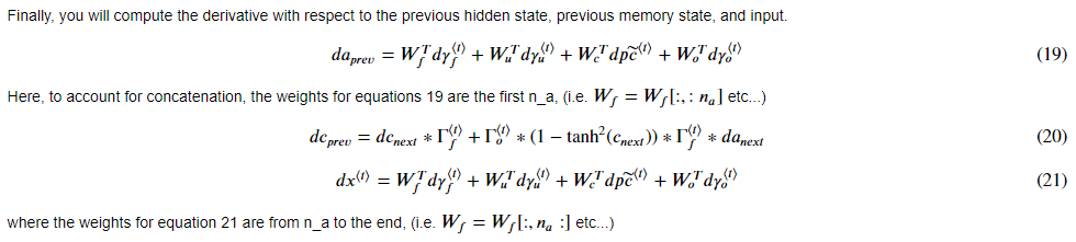
# Compute derivatives w.r.t previous hidden state, previous memory state and input. Use equations (19)-(21). (≈3 lines)
da_prev = np.dot(parameters['Wf'][:, :n_a].T, dft) + np.dot(parameters['Wi'][:, :n_a].T, dit) + np.dot(parameters['Wc'][:, :n_a].T, dcct) + np.dot(parameters['Wo'][:, :n_a].T, dot)
dc_prev = dc_next * ft + ot * (1 - np.square(np.tanh(c_next))) * ft * da_next
dxt = np.dot(parameters['Wf'][:, n_a:].T, dft) + np.dot(parameters['Wi'][:, n_a:].T, dit) + np.dot(parameters['Wc'][:, n_a:].T, dcct) + np.dot(parameters['Wo'][:, n_a:].T, dot)
### END CODE HERE ###
# Save gradients in dictionary
gradients = {"dxt": dxt, "da_prev": da_prev, "dc_prev": dc_prev, "dWf": dWf,"dbf": dbf, "dWi": dWi,"dbi": dbi,
"dWc": dWc,"dbc": dbc, "dWo": dWo,"dbo": dbo}
return gradients
np.random.seed(1)
xt_tmp = np.random.randn(3,10)
a_prev_tmp = np.random.randn(5,10)
c_prev_tmp = np.random.randn(5,10)
parameters_tmp = {}
parameters_tmp['Wf'] = np.random.randn(5, 5+3)
parameters_tmp['bf'] = np.random.randn(5,1)
parameters_tmp['Wi'] = np.random.randn(5, 5+3)
parameters_tmp['bi'] = np.random.randn(5,1)
parameters_tmp['Wo'] = np.random.randn(5, 5+3)
parameters_tmp['bo'] = np.random.randn(5,1)
parameters_tmp['Wc'] = np.random.randn(5, 5+3)
parameters_tmp['bc'] = np.random.randn(5,1)
parameters_tmp['Wy'] = np.random.randn(2,5)
parameters_tmp['by'] = np.random.randn(2,1)

a_next_tmp, c_next_tmp, yt_tmp, cache_tmp = lstm_cell_forward(xt_tmp, a_prev_tmp, c_prev_tmp, parameters_tmp)

da_next_tmp = np.random.randn(5,10)
dc_next_tmp = np.random.randn(5,10)
gradients_tmp = lstm_cell_backward(da_next_tmp, dc_next_tmp, cache_tmp)
print("gradients[\"dxt\"][1][2] =", gradients_tmp["dxt"][1][2])
print("gradients[\"dxt\"].shape =", gradients_tmp["dxt"].shape)
print("gradients[\"da_prev\"][2][3] =", gradients_tmp["da_prev"][2][3])
print("gradients[\"da_prev\"].shape =", gradients_tmp["da_prev"].shape)
print("gradients[\"dc_prev\"][2][3] =", gradients_tmp["dc_prev"][2][3])
print("gradients[\"dc_prev\"].shape =", gradients_tmp["dc_prev"].shape)
print("gradients[\"dWf\"][3][1] =", gradients_tmp["dWf"][3][1])
print("gradients[\"dWf\"].shape =", gradients_tmp["dWf"].shape)
print("gradients[\"dWi\"][1][2] =", gradients_tmp["dWi"][1][2])
print("gradients[\"dWi\"].shape =", gradients_tmp["dWi"].shape)
print("gradients[\"dWc\"][3][1] =", gradients_tmp["dWc"][3][1])
print("gradients[\"dWc\"].shape =", gradients_tmp["dWc"].shape)
print("gradients[\"dWo\"][1][2] =", gradients_tmp["dWo"][1][2])
print("gradients[\"dWo\"].shape =", gradients_tmp["dWo"].shape)
print("gradients[\"dbf\"][4] =", gradients_tmp["dbf"][4])
print("gradients[\"dbf\"].shape =", gradients_tmp["dbf"].shape)
print("gradients[\"dbi\"][4] =", gradients_tmp["dbi"][4])
print("gradients[\"dbi\"].shape =", gradients_tmp["dbi"].shape)
print("gradients[\"dbc\"][4] =", gradients_tmp["dbc"][4])
print("gradients[\"dbc\"].shape =", gradients_tmp["dbc"].shape)
print("gradients[\"dbo\"][4] =", gradients_tmp["dbo"][4])
print("gradients[\"dbo\"].shape =", gradients_tmp["dbo"].shape)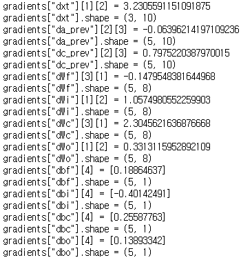
□ Backward Pass through the LSTM RNN
This part is very similar to the rnn_backward function you implemented above. You will first create variables of the same dimension as your return variables. You will then iterate over all the time steps starting from the end and call the one step function you implemented for LSTM at each iteration. You will then update the parameters by summing them individually. Finally return a dictionary with the new gradients.
# UNGRADED FUNCTION: lstm_backward

def lstm_backward(da, caches):

    """
    Implement the backward pass for the RNN with LSTM-cell (over a whole sequence).

    Arguments:
    da -- Gradients w.r.t the hidden states, numpy-array of shape (n_a, m, T_x)
    caches -- cache storing information from the forward pass (lstm_forward)

    Returns:
    gradients -- python dictionary containing:
                        dx -- Gradient of inputs, of shape (n_x, m, T_x)
                        da0 -- Gradient w.r.t. the previous hidden state, numpy array of shape (n_a, m)
                        dWf -- Gradient w.r.t. the weight matrix of the forget gate, numpy array of shape (n_a, n_a + n_x)
                        dWi -- Gradient w.r.t. the weight matrix of the update gate, numpy array of shape (n_a, n_a + n_x)
                        dWc -- Gradient w.r.t. the weight matrix of the memory gate, numpy array of shape (n_a, n_a + n_x)
                        dWo -- Gradient w.r.t. the weight matrix of the output gate, numpy array of shape (n_a, n_a + n_x)
                        dbf -- Gradient w.r.t. biases of the forget gate, of shape (n_a, 1)
                        dbi -- Gradient w.r.t. biases of the update gate, of shape (n_a, 1)
                        dbc -- Gradient w.r.t. biases of the memory gate, of shape (n_a, 1)
                        dbo -- Gradient w.r.t. biases of the output gate, of shape (n_a, 1)
    """

    # Retrieve values from the first cache (t=1) of caches.
    (caches, x) = caches
    (a1, c1, a0, c0, f1, i1, cc1, o1, x1, parameters) = caches[0]

    ### START CODE HERE ###
    # Retrieve dimensions from da's and x1's shapes (≈2 lines)
    n_a, m, T_x = da.shape
    n_x, m = x1.shape

    # initialize the gradients with the right sizes (≈12 lines)
    dx = np.zeros((n_x, m, T_x))
    da0 = np.zeros((n_a, m))
    da_prevt = np.zeros(da0.shape)
    dc_prevt = np.zeros(da0.shape)
    dWf = np.zeros((n_a, n_a + n_x))
    dWi = np.zeros(dWf.shape)
    dWc = np.zeros(dWf.shape)
    dWo = np.zeros(dWf.shape)
    dbf = np.zeros((n_a, 1))
    dbi = np.zeros(dbf.shape)
    dbc = np.zeros(dbf.shape)
    dbo = np.zeros(dbf.shape)

    # loop back over the whole sequence
    for t in reversed(range(T_x)):
        # Compute all gradients using lstm_cell_backward
        gradients = lstm_cell_backward(da[:, :, t], dc_prevt, caches[t])
        # Store or add the gradient to the parameters' previous step's gradient
        da_prevt = gradients["da_prev"]
        dc_prevt = gradients['dc_prev']
        dx[:,:,t] = gradients["dxt"]
        dWf += gradients["dWf"]
        dWi += gradients["dWi"]
        dWc += gradients["dWc"]
        dWo += gradients["dWo"]
        dbf += gradients["dbf"]
        dbi += gradients["dbi"]
        dbc += gradients["dbc"]
        dbo += gradients["dbo"]
    # Set the first activation's gradient to the backpropagated gradient da_prev.
    da0 = da_prevt

    ### END CODE HERE ###

    # Store the gradients in a python dictionary
    gradients = {"dx": dx, "da0": da0, "dWf": dWf,"dbf": dbf, "dWi": dWi,"dbi": dbi,
                "dWc": dWc,"dbc": dbc, "dWo": dWo,"dbo": dbo}

    return gradients
np.random.seed(1)
x_tmp = np.random.randn(3,10,7)
a0_tmp = np.random.randn(5,10)

parameters_tmp = {}
parameters_tmp['Wf'] = np.random.randn(5, 5+3)
parameters_tmp['bf'] = np.random.randn(5,1)
parameters_tmp['Wi'] = np.random.randn(5, 5+3)
parameters_tmp['bi'] = np.random.randn(5,1)
parameters_tmp['Wo'] = np.random.randn(5, 5+3)
parameters_tmp['bo'] = np.random.randn(5,1)
parameters_tmp['Wc'] = np.random.randn(5, 5+3)
parameters_tmp['bc'] = np.random.randn(5,1)
parameters_tmp['Wy'] = np.zeros((2,5))       # unused, but needed for lstm_forward
parameters_tmp['by'] = np.zeros((2,1))       # unused, but needed for lstm_forward

a_tmp, y_tmp, c_tmp, caches_tmp = lstm_forward(x_tmp, a0_tmp, parameters_tmp)

da_tmp = np.random.randn(5, 10, 4)
gradients_tmp = lstm_backward(da_tmp, caches_tmp)

print("gradients[\"dx\"][1][2] =", gradients_tmp["dx"][1][2])
print("gradients[\"dx\"].shape =", gradients_tmp["dx"].shape)
print("gradients[\"da0\"][2][3] =", gradients_tmp["da0"][2][3])
print("gradients[\"da0\"].shape =", gradients_tmp["da0"].shape)
print("gradients[\"dWf\"][3][1] =", gradients_tmp["dWf"][3][1])
print("gradients[\"dWf\"].shape =", gradients_tmp["dWf"].shape)
print("gradients[\"dWi\"][1][2] =", gradients_tmp["dWi"][1][2])
print("gradients[\"dWi\"].shape =", gradients_tmp["dWi"].shape)
print("gradients[\"dWc\"][3][1] =", gradients_tmp["dWc"][3][1])
print("gradients[\"dWc\"].shape =", gradients_tmp["dWc"].shape)
print("gradients[\"dWo\"][1][2] =", gradients_tmp["dWo"][1][2])
print("gradients[\"dWo\"].shape =", gradients_tmp["dWo"].shape)
print("gradients[\"dbf\"][4] =", gradients_tmp["dbf"][4])
print("gradients[\"dbf\"].shape =", gradients_tmp["dbf"].shape)
print("gradients[\"dbi\"][4] =", gradients_tmp["dbi"][4])
print("gradients[\"dbi\"].shape =", gradients_tmp["dbi"].shape)
print("gradients[\"dbc\"][4] =", gradients_tmp["dbc"][4])
print("gradients[\"dbc\"].shape =", gradients_tmp["dbc"].shape)
print("gradients[\"dbo\"][4] =", gradients_tmp["dbo"][4])
print("gradients[\"dbo\"].shape =", gradients_tmp["dbo"].shape)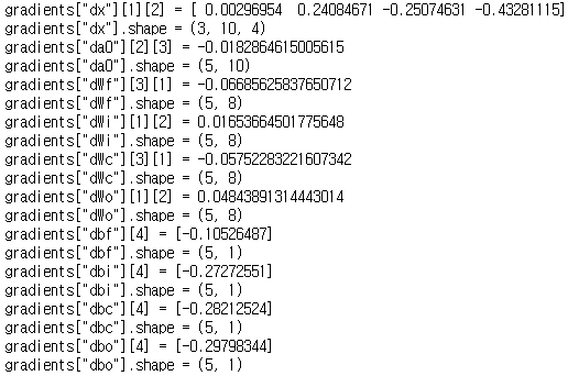
■ 마무리
"Sequence Models" (Andrew Ng)의 1주차 "Building your Recurrent Neural Network - Step by Step"의 실습에 대해서 정리해봤습니다.
그럼 오늘 하루도 즐거운 나날 되길 기도하겠습니다
좋아요와 댓글 부탁드립니다 :)
감사합니다.
'COURSERA' 카테고리의 다른 글
| week 1_Improvise a Jazz Solo with an LSTM Network 실습 (Andrew Ng) (0) | 2022.04.27 |
|---|---|
| week 1_Character level language model - Dinosaurus Island 실습 (Andrew Ng) (0) | 2022.04.27 |
| week 1_Recurrent Neural Networks 연습 문제 (Andrew Ng) (0) | 2022.04.27 |
| week 1_Recurrent Neural Networks (Andrew Ng) (0) | 2022.04.27 |
| [COURSERA] Sequence Models (Andrew Ng) (0) | 2022.03.14 |


댓글