안녕하세요, HELLO
오늘은 DeepLearning.AI에서 진행하는 앤드류 응(Andrew Ng) 교수님의 딥러닝 전문화의 두 번째 과정인 "Improving Deep Neural Networks: Hyperparameter Tuning, Regularization and Optimization"을 정리하려고 합니다.
"Improving Deep Neural Networks: Hyperparameter Tuning, Regularization and Optimization"의 강의 목적은 '랜덤 초기화, L2 및 드롭아웃 정규화, 하이퍼 파라미터 튜닝, 배치 정규화 및 기울기 검사와 같은 표준 신경망 기술' 등을 배우며, 강의는 아래와 같이 구성되어 있습니다.
~ Practical Aspects of Deep Learning
~ Optimization Algorithms
~ Hyperparameter Tuning, Batch Normalization and Programming Frameworks
"Improving Deep Neural Networks" (Andrew Ng)의 3주차 "Tensorflow introduction"의 실습 내용입니다.
By the end of this assignment, you'll be able to do the following in TensorFlow
- Use tf.Variable to modify the state of a variable
- Explain the difference between a variable and a constant
- Train a Neural Network on a TensorFlow dataset
Programming frameworks like TensorFlow not only cut down on time spent coding, but can also perform optimizations that speed up the code itself.
CHAPTER 1. 'Packages'
CHAPTER 2. 'Basic Optimization with GradientTape'
CHAPTER 3. 'Building Your First Neural Network in TensorFlow'
CHAPTER 1. 'Packages'
□ Library
이번 실습에서 사용하게 될 라이브러리 정리입니다.
import h5py
import numpy as np
import tensorflow as tf
import matplotlib.pyplot as plt
from tensorflow.python.framework.ops import EagerTensor
from tensorflow.python.ops.resource_variable_ops import ResourceVariable
import time
CHAPTER 2. 'Basic Optimization with GradientTape'
The beauty of TensorFlow 2 is in its simplicity. Basically, all you need to do is implement forward propagation through a computational graph. TensorFlow will compute the derivatives for you, by moving backwards through the graph recorded with GradientTape. All that's left for you to do then is specify the cost function and optimizer you want to use!
When writing a TensorFlow program, the main object to get used and transformed is the tf.Tensor. These tensors are the TensorFlow equivalent of Numpy arrays, i.e. multidimensional arrays of a given data type that also contain information about the computational graph.
Below, you'll use tf.Variable to store the state of your variables. Variables can only be created once as its initial value defines the variable shape and type. Additionally, the dtype arg in tf.Variable can be set to allow data to be converted to that type. But if none is specified, either the datatype will be kept if the initial value is a Tensor, or convert_to_tensor will decide. It's generally best for you to specify directly, so nothing breaks!
train_dataset = h5py.File('datasets/train_signs.h5', "r")
test_dataset = h5py.File('datasets/test_signs.h5', "r")
x_train = tf.data.Dataset.from_tensor_slices(train_dataset['train_set_x'])
y_train = tf.data.Dataset.from_tensor_slices(train_dataset['train_set_y'])
x_test = tf.data.Dataset.from_tensor_slices(test_dataset['test_set_x'])
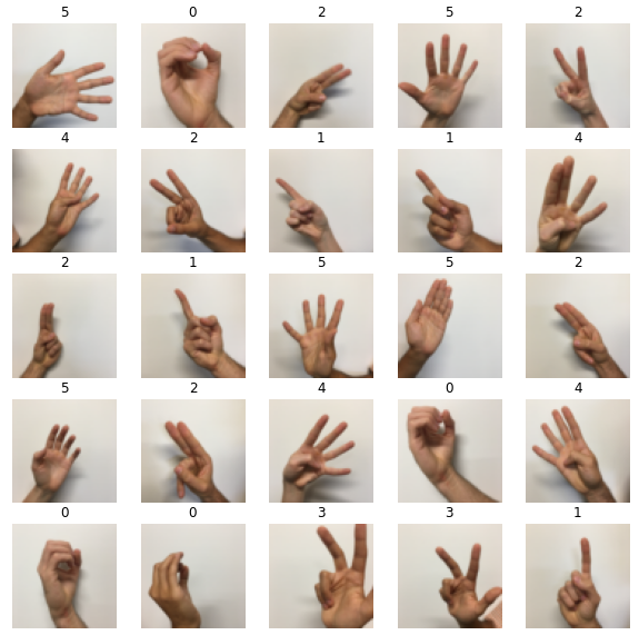
y_test = tf.data.Dataset.from_tensor_slices(test_dataset['test_set_y'])You can see some of the images in the dataset by running the following cell.
images_iter = iter(x_train)
labels_iter = iter(y_train)
plt.figure(figsize=(10, 10))
for i in range(25):
    ax = plt.subplot(5, 5, i + 1)
    plt.imshow(next(images_iter).numpy().astype("uint8"))
    plt.title(next(labels_iter).numpy().astype("uint8"))
    plt.axis("off")
There's one more additional difference between TensorFlow datasets and Numpy arrays: If you need to transform one, you would invoke the map method to apply the function passed as an argument to each of the elements.
□ Linear Function
Let's begin this programming exercise by computing the following equation: 𝑌=𝑊𝑋+𝑏 , where 𝑊 and 𝑋 are random matrices and b is a random vector.
# GRADED FUNCTION: linear_function

def linear_function():
    """
    Implements a linear function:
            Initializes X to be a random tensor of shape (3,1)
            Initializes W to be a random tensor of shape (4,3)
            Initializes b to be a random tensor of shape (4,1)
    Returns:
    result -- Y = WX + b
    """

    np.random.seed(1)

    """
    Note, to ensure that the "random" numbers generated match the expected results,
    please create the variables in the order given in the starting code below.
    (Do not re-arrange the order).
    """
    # (approx. 4 lines)
    # X = ...
    # W = ...
    # b = ...
    # Y = ...
    # YOUR CODE STARTS HERE
    X = tf.constant(np.random.randn(3,1), name = "X")
    W = tf.constant(np.random.randn(4,3), name = "W")
    b = tf.constant(np.random.randn(4,1), name = "b")
    Y = tf.add(tf.matmul(W, X), b)

    # YOUR CODE ENDS HERE
    return Y
result = linear_function()
print(result)

assert type(result) == EagerTensor, "Use the TensorFlow API"
assert np.allclose(result, [[-2.15657382], [ 2.95891446], [-1.08926781], [-0.84538042]]), "Error"
print("\033[92mAll test passed")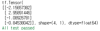
□ Computing the Sigmoid
Amazing! You just implemented a linear function. TensorFlow offers a variety of commonly used neural network functions like tf.sigmoid and tf.softmax.
For this exercise, compute the sigmoid of z.
In this exercise, you will: Cast your tensor to type float32 using tf.cast, then compute the sigmoid using tf.keras.activations.sigmoid
# GRADED FUNCTION: sigmoid

def sigmoid(z):

    """
    Computes the sigmoid of z

    Arguments:
    z -- input value, scalar or vector

    Returns:
    a -- (tf.float32) the sigmoid of z
    """
    # tf.keras.activations.sigmoid requires float16, float32, float64, complex64, or complex128.

    # (approx. 2 lines)
    # z = ...
    # a = ...
    # YOUR CODE STARTS HERE
    z = tf.cast(z, tf.float32)
    a = tf.keras.activations.sigmoid(z)

    # YOUR CODE ENDS HERE
    return a
result = sigmoid(-1)
print ("type: " + str(type(result)))
print ("dtype: " + str(result.dtype))
print ("sigmoid(-1) = " + str(result))
print ("sigmoid(0) = " + str(sigmoid(0.0)))
print ("sigmoid(12) = " + str(sigmoid(12)))

def sigmoid_test(target):
    result = target(0)
    assert(type(result) == EagerTensor)
    assert (result.dtype == tf.float32)
    assert sigmoid(0) == 0.5, "Error"
    assert sigmoid(-1) == 0.26894143, "Error"
    assert sigmoid(12) == 0.9999939, "Error"

    print("\033[92mAll test passed")

sigmoid_test(sigmoid)
□ Using One Hot Encodings
Many times in deep learning you will have a 𝑌 vector with numbers ranging from 00 to 𝐶−1, where 𝐶 is the number of classes. If 𝐶 is for example 4, then you might have the following y vector which you will need to convert like this:
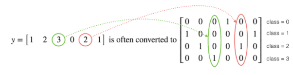
This is called "one hot" encoding, because in the converted representation, exactly one element of each column is "hot" (meaning set to 1). To do this conversion in numpy, you might have to write a few lines of code. In TensorFlow, you can use one line of code
# GRADED FUNCTION: one_hot_matrix
def one_hot_matrix(label, depth=6):
    """
    Computes the one hot encoding for a single label

    Arguments:
        label --  (int) Categorical labels
        depth --  (int) Number of different classes that label can take

    Returns:
         one_hot -- tf.Tensor A single-column matrix with the one hot encoding.
    """
    # (approx. 1 line)
    # one_hot = ...
    # YOUR CODE STARTS HERE
    one_hot = tf.reshape(tf.one_hot(label, depth, axis=0), shape = (depth, ))
    # YOUR CODE ENDS HERE
    return one_hot
def one_hot_matrix_test(target):
    label = tf.constant(1)
    depth = 4
    result = target(label, depth)
    print("Test 1:",result)
    assert result.shape[0] == depth, "Use the parameter depth"
    assert np.allclose(result, [0., 1. ,0., 0.] ), "Wrong output. Use tf.one_hot"
    label_2 = [2]
    result = target(label_2, depth)
    print("Test 2:", result)
    assert result.shape[0] == depth, "Use the parameter depth"
    assert np.allclose(result, [0., 0. ,1., 0.] ), "Wrong output. Use tf.reshape as instructed"

    print("\033[92mAll test passed")

one_hot_matrix_test(one_hot_matrix)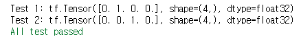
□ Initialize the Parameters
Now you'll initialize a vector of numbers with the Glorot initializer. The function you'll be calling is tf.keras.initializers.GlorotNormal, which draws samples from a truncated normal distribution centered on 0, with stddev = sqrt(2 / (fan_in + fan_out)), where fan_in is the number of input units and fan_out is the number of output units, both in the weight tensor.
To initialize with zeros or ones you could use tf.zeros() or tf.ones() instead.
# GRADED FUNCTION: initialize_parameters

def initialize_parameters():
    """
    Initializes parameters to build a neural network with TensorFlow. The shapes are:
                        W1 : [25, 12288]
                        b1 : [25, 1]
                        W2 : [12, 25]
                        b2 : [12, 1]
                        W3 : [6, 12]
                        b3 : [6, 1]

    Returns:
    parameters -- a dictionary of tensors containing W1, b1, W2, b2, W3, b3
    """

    initializer = tf.keras.initializers.GlorotNormal(seed=1)
    #(approx. 6 lines of code)
    # W1 = ...
    # b1 = ...
    # W2 = ...
    # b2 = ...
    # W3 = ...
    # b3 = ...
    # YOUR CODE STARTS HERE
    W1 = tf.Variable(initializer(shape=(25, 12288)))
    b1 = tf.Variable(initializer(shape=(25, 1)))
    W2 = tf.Variable(initializer(shape=(12, 25)))
    b2 = tf.Variable(initializer(shape=(12, 1)))
    W3 = tf.Variable(initializer(shape=(6, 12)))
    b3 = tf.Variable(initializer(shape=(6, 1)))

    # YOUR CODE ENDS HERE

    parameters = {"W1": W1,
                  "b1": b1,
                  "W2": W2,
                  "b2": b2,
                  "W3": W3,
                  "b3": b3}

    return parameters
def initialize_parameters_test(target):
    parameters = target()

    values = {"W1": (25, 12288),
              "b1": (25, 1),
              "W2": (12, 25),
              "b2": (12, 1),
              "W3": (6, 12),
              "b3": (6, 1)}

    for key in parameters:
        print(f"{key} shape: {tuple(parameters[key].shape)}")
        assert type(parameters[key]) == ResourceVariable, "All parameter must be created using tf.Variable"
        assert tuple(parameters[key].shape) == values[key], f"{key}: wrong shape"
        assert np.abs(np.mean(parameters[key].numpy())) < 0.5,  f"{key}: Use the GlorotNormal initializer"
        assert np.std(parameters[key].numpy()) > 0 and np.std(parameters[key].numpy()) < 1, f"{key}: Use the GlorotNormal initializer"

    print("\033[92mAll test passed")

initialize_parameters_test(initialize_parameters)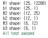
parameters = initialize_parameters()
CHAPTER 3. 'Building Your First Neural Network in TensorFlow'
In this part of the assignment you will build a neural network using TensorFlow. Remember that there are two parts to implementing a TensorFlow model:
- Implement forward propagation
- Retrieve the gradients and train the model
□ Implement Forward Propagation
One of TensorFlow's great strengths lies in the fact that you only need to implement the forward propagation function and it will keep track of the operations you did to calculate the back propagation automatically.
□ forward_propagation
# GRADED FUNCTION: forward_propagation

def forward_propagation(X, parameters):
    """
    Implements the forward propagation for the model: LINEAR -> RELU -> LINEAR -> RELU -> LINEAR

    Arguments:
    X -- input dataset placeholder, of shape (input size, number of examples)
    parameters -- python dictionary containing your parameters "W1", "b1", "W2", "b2", "W3", "b3"
                  the shapes are given in initialize_parameters

    Returns:
    Z3 -- the output of the last LINEAR unit
    """

    # Retrieve the parameters from the dictionary "parameters"
    W1 = parameters['W1']
    b1 = parameters['b1']
    W2 = parameters['W2']
    b2 = parameters['b2']
    W3 = parameters['W3']
    b3 = parameters['b3']

    #(approx. 5 lines)                   # Numpy Equivalents:
    # Z1 = ...                           # Z1 = np.dot(W1, X) + b1
    # A1 = ...                           # A1 = relu(Z1)
    # Z2 = ...                           # Z2 = np.dot(W2, A1) + b2
    # A2 = ...                           # A2 = relu(Z2)
    # Z3 = ...                           # Z3 = np.dot(W3, A2) + b3
    # YOUR CODE STARTS HERE
    Z1 = tf.math.add(tf.linalg.matmul(W1, X), b1)
    A1 = tf.keras.activations.relu(Z1)
    Z2 = tf.math.add(tf.linalg.matmul(W2, A1), b2)
    A2 = tf.keras.activations.relu(Z2)
    Z3 = tf.math.add(tf.linalg.matmul(W3, A2), b3)

    # YOUR CODE ENDS HERE

    return Z3
def forward_propagation_test(target, examples):
    minibatches = examples.batch(2)
    for minibatch in minibatches:
        forward_pass = target(tf.transpose(minibatch), parameters)
        print(forward_pass)
        assert type(forward_pass) == EagerTensor, "Your output is not a tensor"
        assert forward_pass.shape == (6, 2), "Last layer must use W3 and b3"
        assert np.allclose(forward_pass,
                            [[-0.13430887,  0.14086473],
                             [ 0.21588647, -0.02582335],
                             [ 0.7059658,   0.6484556 ],
                             [-1.1260961,  -0.9329492 ],
                             [-0.20181894, -0.3382722 ],
                             [ 0.9558965,   0.94167566]]), "Output does not match"
        break


    print("\033[92mAll test passed")

forward_propagation_test(forward_propagation, new_train)
□ Compute the Cost
All you have to do now is define the loss function that you're going to use. For this case, since we have a classification problem with 6 labels, a categorical cross entropy will work!
# GRADED FUNCTION: compute_cost

def compute_cost(logits, labels):
    """
    Computes the cost

    Arguments:
    logits -- output of forward propagation (output of the last LINEAR unit), of shape (6, num_examples)
    labels -- "true" labels vector, same shape as Z3

    Returns:
    cost - Tensor of the cost function
    """

    #(1 line of code)
    # cost = ...
    # YOUR CODE STARTS HERE
    cost = tf.reduce_mean(tf.keras.losses.categorical_crossentropy(labels, logits))

    # YOUR CODE ENDS HERE
    return cost
□ Train the Model
Let's talk optimizers. You'll specify the type of optimizer in one line, in this case tf.keras.optimizers.Adam (though you can use others such as SGD), and then call it within the training loop.
Notice the tape.gradient function: this allows you to retrieve the operations recorded for automatic differentiation inside the GradientTape block. Then, calling the optimizer method apply_gradients, will apply the optimizer's update rules to each trainable parameter. At the end of this assignment, you'll find some documentation that explains this more in detail, but for now, a simple explanation will do. ;)
Here you should take note of an important extra step that's been added to the batch training process:
tf.Data.dataset = dataset.prefetch(8)
What this does is prevent a memory bottleneck that can occur when reading from disk. prefetch() sets aside some data and keeps it ready for when it's needed. It does this by creating a source dataset from your input data, applying a transformation to preprocess the data, then iterating over the dataset the specified number of elements at a time. This works because the iteration is streaming, so the data doesn't need to fit into the memory.
def model(X_train, Y_train, X_test, Y_test, learning_rate = 0.0001,
          num_epochs = 1500, minibatch_size = 32, print_cost = True):
    """
    Implements a three-layer tensorflow neural network: LINEAR->RELU->LINEAR->RELU->LINEAR->SOFTMAX.

    Arguments:
    X_train -- training set, of shape (input size = 12288, number of training examples = 1080)
    Y_train -- test set, of shape (output size = 6, number of training examples = 1080)
    X_test -- training set, of shape (input size = 12288, number of training examples = 120)
    Y_test -- test set, of shape (output size = 6, number of test examples = 120)
    learning_rate -- learning rate of the optimization
    num_epochs -- number of epochs of the optimization loop
    minibatch_size -- size of a minibatch
    print_cost -- True to print the cost every 10 epochs

    Returns:
    parameters -- parameters learnt by the model. They can then be used to predict.
    """

    costs = []                                        # To keep track of the cost
    train_acc = []
    test_acc = []

    # Initialize your parameters
    #(1 line)
    parameters = initialize_parameters()

    W1 = parameters['W1']
    b1 = parameters['b1']
    W2 = parameters['W2']
    b2 = parameters['b2']
    W3 = parameters['W3']
    b3 = parameters['b3']

    optimizer = tf.keras.optimizers.Adam(learning_rate)

    # The CategoricalAccuracy will track the accuracy for this multiclass problem
    test_accuracy = tf.keras.metrics.CategoricalAccuracy()
    train_accuracy = tf.keras.metrics.CategoricalAccuracy()

    dataset = tf.data.Dataset.zip((X_train, Y_train))
    test_dataset = tf.data.Dataset.zip((X_test, Y_test))

    # We can get the number of elements of a dataset using the cardinality method
    m = dataset.cardinality().numpy()

    minibatches = dataset.batch(minibatch_size).prefetch(8)
    test_minibatches = test_dataset.batch(minibatch_size).prefetch(8)
    #X_train = X_train.batch(minibatch_size, drop_remainder=True).prefetch(8)# <<< extra step
    #Y_train = Y_train.batch(minibatch_size, drop_remainder=True).prefetch(8) # loads memory faster

    # Do the training loop
    for epoch in range(num_epochs):

        epoch_cost = 0.

        #We need to reset object to start measuring from 0 the accuracy each epoch
        train_accuracy.reset_states()

        for (minibatch_X, minibatch_Y) in minibatches:

            with tf.GradientTape() as tape:
                # 1. predict
                Z3 = forward_propagation(tf.transpose(minibatch_X), parameters)

                # 2. loss
                minibatch_cost = compute_cost(Z3, tf.transpose(minibatch_Y))

            # We acumulate the accuracy of all the batches
            train_accuracy.update_state(tf.transpose(Z3), minibatch_Y)

            trainable_variables = [W1, b1, W2, b2, W3, b3]
            grads = tape.gradient(minibatch_cost, trainable_variables)
            optimizer.apply_gradients(zip(grads, trainable_variables))
            epoch_cost += minibatch_cost

        # We divide the epoch cost over the number of samples
        epoch_cost /= m

        # Print the cost every 10 epochs
        if print_cost == True and epoch % 10 == 0:
            print ("Cost after epoch %i: %f" % (epoch, epoch_cost))
            print("Train accuracy:", train_accuracy.result())

            # We evaluate the test set every 10 epochs to avoid computational overhead
            for (minibatch_X, minibatch_Y) in test_minibatches:
                Z3 = forward_propagation(tf.transpose(minibatch_X), parameters)
                test_accuracy.update_state(tf.transpose(Z3), minibatch_Y)
            print("Test_accuracy:", test_accuracy.result())

            costs.append(epoch_cost)
            train_acc.append(train_accuracy.result())
            test_acc.append(test_accuracy.result())
            test_accuracy.reset_states()


    return parameters, costs, train_acc, test_acc
parameters, costs, train_acc, test_acc = model(new_train, new_y_train, new_test, new_y_test, num_epochs=100)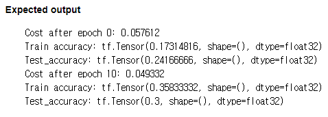
# Plot the cost
plt.plot(np.squeeze(costs))
plt.ylabel('cost')
plt.xlabel('iterations (per fives)')
plt.title("Learning rate =" + str(0.0001))
plt.show()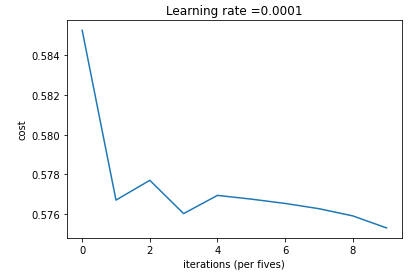
# Plot the train accuracy
plt.plot(np.squeeze(train_acc))
plt.ylabel('Train Accuracy')
plt.xlabel('iterations (per fives)')
plt.title("Learning rate =" + str(0.0001))
# Plot the test accuracy
plt.plot(np.squeeze(test_acc))
plt.ylabel('Test Accuracy')
plt.xlabel('iterations (per fives)')
plt.title("Learning rate =" + str(0.0001))
plt.show()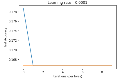
Here's a quick recap of all you just achieved:
- Used tf.Variable to modify your variables
- Trained a Neural Network on a TensorFlow dataset
You are now able to harness the power of TensorFlow to create cool things, faster. Nice!
■ 마무리
"Improving Deep Neural Networks" (Andrew Ng)의 3주차 "Tensorflow introduction"의 실습 내용에 대해서 정리해봤습니다.
그럼 오늘 하루도 즐거운 나날 되길 기도하겠습니다
좋아요와 댓글 부탁드립니다 :)
감사합니다.


댓글