
안녕하세요, HELLO
오늘은 DeepLearning.AI, Amazon Web Services에서 진행하는 Practical Data Science Specialization의 첫 번째 과정인 "Analyze Datasets and Train ML Models using AutoML"을 정리하려고 합니다.
"Analyze Datasets and Train ML Models using AutoML"의 강의를 통해 'exploratory data analysis (EDA), automated machine learning (AutoML), and text classification algorithms에 대해서 배우게 됩니다. 강의는 아래와 같이 구성되어 있습니다.
~ Explore the Use Case and Analyze the Dataset
~ Data Bias and Feature Importance
~ Use Automated Machine Learning to train a Text Classifier
~ Built-in algorithms
"Analyze Datasets and Train ML Models using AutoML"의 1주차 "Register and visualize dataset"의 실습 내용입니다.
■ Introduction
In this lab you will ingest and transform the customer product reviews dataset. Then you will use AWS data stack services such as AWS Glue and Amazon Athena for ingesting and querying the dataset. Finally you will use AWS Data Wrangler to analyze the dataset and plot some visuals extracting insights.
CHAPTER 1. 'Ingest and transform the public dataset'
CHAPTER 2. 'Register the public dataset for querying and visualizing'
CHAPTER 3. 'Visualize data'
CHAPTER 1. 'Ingest and transform the public dataset'
The AWS Command Line Interface (CLI) is a unified tool to manage your AWS services. With just one tool, you can control multiple AWS services from the command line and automate them through scripts. You will use it to list the dataset files.
aws s3 ls [bucket_name] function lists all objects in the S3 bucket. Let's use it to view the reviews data files in CSV format:
□ Exercise 1
View the list of the files available in the public bucket s3://dlai-practical-data-science/data/raw/.
### BEGIN SOLUTION - DO NOT delete this comment for grading purposes
!aws s3 ls s3://dlai-practical-data-science/data/raw/ # Replace None
### END SOLUTION - DO NOT delete this comment for grading purposes

# EXPECTED OUTPUT
# ... womens_clothing_ecommerce_reviews.csv
□ Copy the data locally to the notebook
aws s3 cp [bucket_name/file_name] [file_name] function copies the file from the S3 bucket into the local environment or into another S3 bucket. Let's use it to copy the file with the dataset locally.
!aws s3 cp s3://dlai-practical-data-science/data/raw/womens_clothing_ecommerce_reviews.csv ./womens_clothing_ecommerce_reviews.csv
Now use the Pandas dataframe to load and preview the data.
import pandas as pd
import csv

df = pd.read_csv('./womens_clothing_ecommerce_reviews.csv',
                 index_col=0)

df.shape
□ Transform the data
To simplify the task, you will transform the data into a comma-separated value (CSV) file that contains only a review_body, product_category, and sentiment derived from the original data.
df_transformed = df.rename(columns={'Review Text': 'review_body',
                                    'Rating': 'star_rating',
                                    'Class Name': 'product_category'})
df_transformed.drop(columns=['Clothing ID', 'Age', 'Title', 'Recommended IND', 'Positive Feedback Count', 'Division Name', 'Department Name'],
                    inplace=True)

df_transformed.dropna(inplace=True)

df_transformed.shape

# (22628, 3)
Now convert the star_rating into the sentiment (positive, neutral, negative), which later on will be for the prediction.
def to_sentiment(star_rating):
    if star_rating in {1, 2}: # negative
        return -1
    if star_rating == 3:      # neutral
        return 0
    if star_rating in {4, 5}: # positive
        return 1

# transform star_rating into the sentiment
df_transformed['sentiment'] = df_transformed['star_rating'].apply(lambda star_rating:
    to_sentiment(star_rating=star_rating)
)

# drop the star rating column
df_transformed.drop(columns=['star_rating'],
                    inplace=True)

# remove reviews for product_categories with < 10 reviews
df_transformed = df_transformed.groupby('product_category').filter(lambda reviews : len(reviews) > 10)[['sentiment', 'review_body', 'product_category']]

df_transformed.shape

# (22626, 3)
# preview the results
df_transformed
□ Write the data to a CSV file
df_transformed.to_csv('./womens_clothing_ecommerce_reviews_transformed.csv',
                      index=False)
CHAPTER 2. 'Register the public dataset for querying and visualizing'
You will register the public dataset into an S3-backed database table so you can query and visualize our dataset at scale.
□ Register S3 dataset files as a table for querying
Let's import required modules.
boto3 is the AWS SDK for Python to create, configure, and manage AWS services, such as Amazon Elastic Compute Cloud (Amazon EC2) and Amazon Simple Storage Service (Amazon S3). The SDK provides an object-oriented API as well as low-level access to AWS services.
sagemaker is the SageMaker Python SDK which provides several high-level abstractions for working with the Amazon SageMaker.
import boto3 #  AWS SDK for Python to create, configure, and manage AWS services
import sagemaker # several high-level abstractions for working with the Amazon SageMaker.
import pandas as pd
import numpy as np
import botocore

config = botocore.config.Config(user_agent_extra='dlai-pds/c1/w1')

# low-level service client of the boto3 session
sm = boto3.client(service_name='sagemaker',
                  config=config)

sess = sagemaker.Session(sagemaker_client=sm)

bucket = sess.default_bucket()
role = sagemaker.get_execution_role()
region = sess.boto_region_name
account_id = sess.account_id

print('S3 Bucket: {}'.format(bucket))
print('Region: {}'.format(region))
print('Account ID: {}'.format(account_id))
Review the empty bucket which was created automatically for this account.
Instructions:
- open the link (실습에서는 과정에 따라, 진행 과정을 링크로 확인할 수 있습니다)
- click on the S3 bucket name sagemaker-us-east-1-ACCOUNT
- check that it is empty at this stage
Copy the file into the S3 bucket.
!aws s3 cp ./womens_clothing_ecommerce_reviews_transformed.csv s3://$bucket/data/transformed/womens_clothing_ecommerce_reviews_transformed.csvReview the bucket with the file we uploaded above.
Instructions:
- open the link (실습에서는 과정에 따라, 진행 과정을 링크로 확인할 수 있습니다)
- check that the CSV file is located in the S3 bucket
- check the location directory structure is the same as in the CLI command above
- click on the file name and see the available information about the file (region, size, S3 URI, Amazon Resource Name (ARN))
■ Import AWS Data Wrangler
AWS Data Wrangler is an AWS Professional Service open source python initiative that extends the power of Pandas library to AWS connecting dataframes and AWS data related services (Amazon Redshift, AWS Glue, Amazon Athena, Amazon EMR, Amazon QuickSight, etc).
Built on top of other open-source projects like Pandas, Apache Arrow, Boto3, SQLAlchemy, Psycopg2 and PyMySQL, it offers abstracted functions to execute usual ETL tasks like load/unload data from data lakes, data warehouses and databases.
Review the AWS Data Wrangler documentation: https://aws-data-wrangler.readthedocs.io/en/stable/
import awswrangler as wr
■ Create AWS Glue Catalog database
The data catalog features of AWS Glue and the inbuilt integration to Amazon S3 simplify the process of identifying data and deriving the schema definition out of the discovered data. Using AWS Glue crawlers within your data catalog, you can traverse your data stored in Amazon S3 and build out the metadata tables that are defined in your data catalog.
Here you will use wr.catalog.create_database function to create a database with the name dsoaws_deep_learning ("dsoaws" stands for "Data Science on AWS").
wr.catalog.create_database(
    name='dsoaws_deep_learning',
    exist_ok=True
)

dbs = wr.catalog.get_databases()

for db in dbs:
    print("Database name: " + db['Name'])

# Database name: dsoaws_deep_learning
Review the created database in the AWS Glue Catalog.
Instructions:
- open the link (실습에서는 과정에 따라, 진행 과정을 링크로 확인할 수 있습니다)
- on the left side panel notice that you are in the AWS Glue -> Data Catalog -> Databases
- check that the database dsoaws_deep_learning has been created
- click on the name of the database
- click on the Tables in dsoaws_deep_learning link to see that there are no tables
Register CSV data with AWS Glue Catalog
res = wr.catalog.create_csv_table(
    database='...', # AWS Glue Catalog database name
    path='s3://{}/data/transformed/'.format(bucket), # S3 object path for the data
    table='reviews', # registered table name
    columns_types={
        'sentiment': 'int',
        'review_body': 'string',
        'product_category': 'string'
    },
    mode='overwrite',
    skip_header_line_count=1,
    sep=','
)
wr.catalog.create_csv_table(
### BEGIN SOLUTION - DO NOT delete this comment for grading purposes
database='dsoaws_deep_learning', # Replace None
### END SOLUTION - DO NOT delete this comment for grading purposes
path='s3://{}/data/transformed/'.format(bucket),
table="reviews",
columns_types={
'sentiment': 'int',
'review_body': 'string',
'product_category': 'string'
},
mode='overwrite',
skip_header_line_count=1,
sep=','
)Review the registered table in the AWS Glue Catalog.
Instructions:
- open the link (실습에서는 과정에 따라, 진행 과정을 링크로 확인할 수 있습니다)
- on the left side panel notice that you are in the AWS Glue -> Data Catalog -> Databases -> Tables
- check that you can see the table reviews from the database dsoaws_deep_learning in the list
- click on the name of the table
- explore the available information about the table (name, database, classification, location, schema etc.)
Review the table shape:
table = wr.catalog.table(database='dsoaws_deep_learning',
                         table='reviews')
table
□ Create default S3 bucket for Amazon Athena
Amazon Athena requires this S3 bucket to store temporary query results and improve performance of subsequent queries. The contents of this bucket are mostly binary and human-unreadable.
# S3 bucket name
wr.athena.create_athena_bucket()

# EXPECTED OUTPUT
# 's3://aws-athena-query-results-ACCOUNT-REGION/'
CHAPTER 3. 'Visualize data'
Reviews dataset - column descriptions
- sentiment: The review's sentiment (-1, 0, 1).
- product_category: Broad product category that can be used to group reviews (in this case digital videos).
- review_body: The text of the review.
□ Preparation for data visualization
■ Imports
import numpy as np
import seaborn as sns

import matplotlib.pyplot as plt
%matplotlib inline
%config InlineBackend.figure_format='retina'
■ Settings
Set AWS Glue database and table name. And set seaborn parameters.
# Do not change the database and table names - they are used for grading purposes!
database_name = 'dsoaws_deep_learning'
table_name = 'reviews'

sns.set_style = 'seaborn-whitegrid'

sns.set(rc={"font.style":"normal",
            "axes.facecolor":"white",
            'grid.color': '.8',
            'grid.linestyle': '-',
            "figure.facecolor":"white",
            "figure.titlesize":20,
            "text.color":"black",
            "xtick.color":"black",
            "ytick.color":"black",
            "axes.labelcolor":"black",
            "axes.grid":True,
            'axes.labelsize':10,
            'xtick.labelsize':10,
            'font.size':10,
            'ytick.labelsize':10})
■ Run SQL queries using Amazon Athena
Amazon Athena lets you query data in Amazon S3 using a standard SQL interface. It reflects the databases and tables in the AWS Glue Catalog. You can create interactive queries and perform any data manipulations required for further downstream processing.
Standard SQL query can be saved as a string and then passed as a parameter into the Athena query. Run the following cells as an example to count the total number of reviews by sentiment. The SQL query here will take the following form:
SELECT column_name, COUNT(column_name) as new_column_name
FROM table_name
GROUP BY column_name
ORDER BY column_name
If you are not familiar with the SQL query statements, you can review some tutorials following the link.
□ How many reviews per sentiment?
Set the SQL statement to find the count of sentiments:
statement_count_by_sentiment = """
SELECT sentiment, COUNT(sentiment) AS count_sentiment
FROM reviews
GROUP BY sentiment
ORDER BY sentiment
"""

df_count_by_sentiment = wr.athena.read_sql_query(
    sql=statement_count_by_sentiment,
    database=database_name
)

print(df_count_by_sentiment)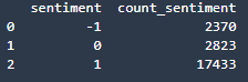
Preview the results of the query:
df_count_by_sentiment.plot(kind='bar', x='sentiment', y='count_sentiment', rot=0)
□ Exercise 3
Use Amazon Athena query with the standard SQL statement passed as a parameter, to calculate the total number of reviews per product_category in the table reviews.
Instructions: Pass the SQL statement of the form
SELECT category_column, COUNT(column_name) AS new_column_name
FROM table_name
GROUP BY category_column
ORDER BY new_column_name DESC
as a triple quote string into the variable statement_count_by_category. Please use the column sentiment in the COUNT function and give it a new name count_sentiment.
# Replace all None
### BEGIN SOLUTION - DO NOT delete this comment for grading purposes
statement_count_by_category = """
SELECT product_category, COUNT(sentiment) AS count_sentiment
FROM reviews
GROUP BY product_category
ORDER BY count_sentiment DESC
"""
### END SOLUTION - DO NOT delete this comment for grading purposes
%%time
df_count_by_category = wr.athena.read_sql_query(
    sql=statement_count_by_category,
    database=database_name
)

df_count_by_category

# EXPECTED OUTPUT
# Dresses: 6145
# Knits: 4626
# Blouses: 2983
# Sweaters: 1380
# Pants: 1350
# ...
□ Which product categories are highest rated by average sentiment?
Set the SQL statement to find the average sentiment per product category, showing the results in the descending order:
statement_avg_by_category = """
SELECT product_category, AVG(sentiment) AS avg_sentiment
FROM {}
GROUP BY product_category
ORDER BY avg_sentiment DESC
""".format(table_name)
Query data in Amazon Athena database passing the prepared SQL statement:
%%time
df_avg_by_category = wr.athena.read_sql_query(
    sql=statement_avg_by_category,
    database=database_name
)
Preview the query results in the temporary S3 bucket: s3://aws-athena-query-results-ACCOUNT-REGION/
Instructions:
- open the link
- check the name of the S3 bucket
- briefly check the content of it
df_avg_by_category
□ Visualization
def show_values_barplot(axs, space):
    def _show_on_plot(ax):
        for p in ax.patches:
            _x = p.get_x() + p.get_width() + float(space)
            _y = p.get_y() + p.get_height()
            value = round(float(p.get_width()),2)
            ax.text(_x, _y, value, ha="left")

    if isinstance(axs, np.ndarray):
        for idx, ax in np.ndenumerate(axs):
            _show_on_plot(ax)
    else:
        _show_on_plot(axs)
# Create plot
barplot = sns.barplot(
    data = df_avg_by_category,
    y='product_category',
    x='avg_sentiment',
    color="b",
    saturation=1
)

# Set the size of the figure
sns.set(rc={'figure.figsize':(15.0, 10.0)})

# Set title and x-axis ticks
plt.title('Average sentiment by product category')
#plt.xticks([-1, 0, 1], ['Negative', 'Neutral', 'Positive'])

# Helper code to show actual values afters bars
show_values_barplot(barplot, 0.1)

plt.xlabel("Average sentiment")
plt.ylabel("Product category")

plt.tight_layout()
# Do not change the figure name - it is used for grading purposes!
plt.savefig('avg_sentiment_per_category.png', dpi=300)

# Show graphic
plt.show(barplot)
□ Which product categories have the most reviews?
Set the SQL statement to find the count of sentiment per product category, showing the results in the descending order:
statement_count_by_category_desc = """
SELECT product_category, COUNT(*) AS count_reviews
FROM {}
GROUP BY product_category
ORDER BY count_reviews DESC
""".format(table_name)
Query data in Amazon Athena database passing the prepared SQL statement:
%%time
df_count_by_category_desc = wr.athena.read_sql_query(
    sql=statement_count_by_category_desc,
    database=database_name
)

# Store maximum number of sentiment for the visualization plot:

max_sentiment = df_count_by_category_desc['count_reviews'].max()
print('Highest number of reviews (in a single category): {}'.format(max_sentiment))

# Highest number of reviews (in a single category): 6145
□ Exercise 4
Use barplot function to plot number of reviews per product category.
Instructions: Use the barplot chart example in the previous section, passing the newly defined dataframe df_count_by_category_desc with the count of reviews. Here, please put the product_category column into the y argument.
# Create seaborn barplot
barplot = sns.barplot(
    ### BEGIN SOLUTION - DO NOT delete this comment for grading purposes
    data=df_count_by_category_desc, # Replace None
    y='product_category', # Replace None
    x='count_reviews', # Replace None
    ### END SOLUTION - DO NOT delete this comment for grading purposes
    color="b",
    saturation=1
)

# Set the size of the figure
sns.set(rc={'figure.figsize':(15.0, 10.0)})

# Set title
plt.title("Number of reviews per product category")
plt.xlabel("Number of reviews")
plt.ylabel("Product category")

plt.tight_layout()

# Do not change the figure name - it is used for grading purposes!
plt.savefig('num_reviews_per_category.png', dpi=300)

# Show the barplot
plt.show(barplot)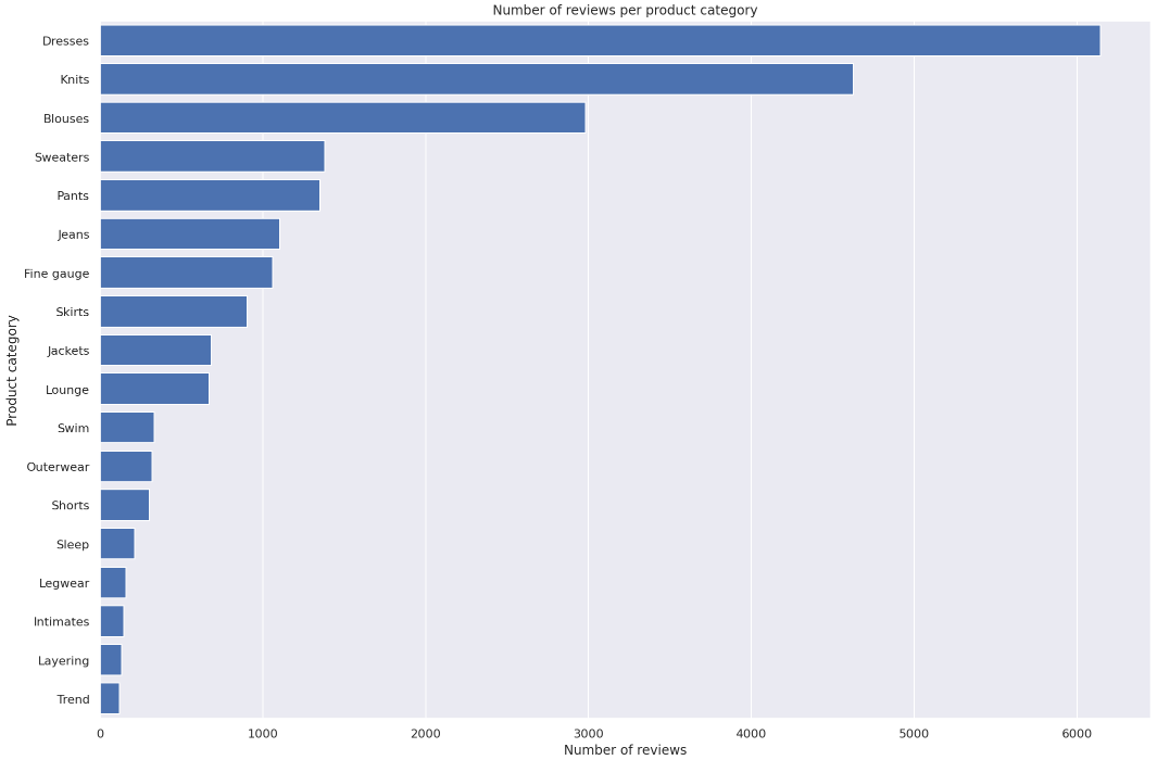
□ What is the breakdown of sentiments per product category
Set the SQL statement to find the count of sentiment per product category and sentiment:
statement_count_by_category_and_sentiment = """
SELECT product_category,
         sentiment,
         COUNT(*) AS count_reviews
FROM {}
GROUP BY  product_category, sentiment
ORDER BY  product_category ASC, sentiment DESC, count_reviews
""".format(table_name)

# Query data in Amazon Athena database passing the prepared SQL statement:

df_count_by_category_and_sentiment = wr.athena.read_sql_query(
    sql=statement_count_by_category_and_sentiment,
    database=database_name
)
Prepare for stacked percentage horizontal bar plot showing proportion of sentiments per product category.
# Create grouped dataframes by category and by sentiment
grouped_category = df_count_by_category_and_sentiment.groupby('product_category')
grouped_star = df_count_by_category_and_sentiment.groupby('sentiment')

# Create sum of sentiments per star sentiment
df_sum = df_count_by_category_and_sentiment.groupby(['sentiment']).sum()

# Calculate total number of sentiments
total = df_sum['count_reviews'].sum()
print('Total number of reviews: {}'.format(total))

# Total number of reviews: 22626
Create dictionary of product categories and array of star rating distribution per category.
distribution = {}
count_reviews_per_star = []
i=0

for category, sentiments in grouped_category:
    count_reviews_per_star = []
    for star in sentiments['sentiment']:
        count_reviews_per_star.append(sentiments.at[i, 'count_reviews'])
        i=i+1;
    distribution[category] = count_reviews_per_star
Build array per star across all categories.
distribution
df_distribution_pct = pd.DataFrame(distribution).transpose().apply(
    lambda num_sentiments: num_sentiments/sum(num_sentiments)*100, axis=1
)
df_distribution_pct.columns=['1', '0', '-1']
df_distribution_pct
□ Visualization
Plot the distributions of sentiments per product category.
categories = df_distribution_pct.index

# Plot bars
plt.figure(figsize=(10,5))

df_distribution_pct.plot(kind="barh",
                         stacked=True,
                         edgecolor='white',
                         width=1.0,
                         color=['green',
                                'orange',
                                'blue'])

plt.title("Distribution of reviews per sentiment per category",
          fontsize='16')

plt.legend(bbox_to_anchor=(1.04,1),
           loc="upper left",
           labels=['Positive',
                   'Neutral',
                   'Negative'])

plt.xlabel("% Breakdown of sentiments", fontsize='14')
plt.gca().invert_yaxis()
plt.tight_layout()

# Do not change the figure name - it is used for grading purposes!
plt.savefig('distribution_sentiment_per_category.png', dpi=300)
plt.show()
□ Analyze the distribution of review word counts
Set the SQL statement to count the number of the words in each of the reviews:
statement_num_words = """
    SELECT CARDINALITY(SPLIT(review_body, ' ')) as num_words
    FROM {}
""".format(table_name)

# Query data in Amazon Athena database passing the SQL statement:

df_num_words = wr.athena.read_sql_query(
    sql=statement_num_words,
    database=database_name
)
Print out and analyse some descriptive statistics:
summary = df_num_words["num_words"].describe(percentiles=[0.10, 0.20, 0.30, 0.40, 0.50, 0.60, 0.70, 0.80, 0.90, 1.00])
summary
Plot the distribution of the words number per review:
df_num_words["num_words"].plot.hist(xticks=[0, 16, 32, 64, 128, 256], bins=100, range=[0, 256]).axvline(
    x=summary["100%"], c="red"
)

plt.xlabel("Words number", fontsize='14')
plt.ylabel("Frequency", fontsize='14')
plt.savefig('distribution_num_words_per_review.png', dpi=300)
plt.show()
■ 마무리
"Analyze Datasets and Train ML Models using AutoML"의 1주차 "Register and visualize dataset"의 실습에 대해서 정리해봤습니다.
그럼 오늘 하루도 즐거운 나날 되길 기도하겠습니다
좋아요와 댓글 부탁드립니다 :)
감사합니다.
'COURSERA' 카테고리의 다른 글
| week 1_Feature Engineering and Feature Store 연습 문제 (0) | 2022.07.10 |
|---|---|
| week 1_Feature Engineering and Feature Store (0) | 2022.07.10 |
| week 1_Explore the Use Case and Analyze the Dataset 연습 문제 (0) | 2022.05.21 |
| week 1_Explore the Use Case and Analyze the Dataset (0) | 2022.05.21 |
| [COURSERA] Build, Train, and Deploy ML Pipelines using BERT (Amazon Web Services) (0) | 2022.05.17 |


댓글