안녕하세요, HELLO
오늘은 DeepLearning.AI에서 진행하는 앤드류 응(Andrew Ng) 교수님의 딥러닝 전문화의 두 번째 과정인 "Improving Deep Neural Networks: Hyperparameter Tuning, Regularization and Optimization"을 정리하려고 합니다.
"Improving Deep Neural Networks: Hyperparameter Tuning, Regularization and Optimization"의 강의 목적은 '랜덤 초기화, L2 및 드롭아웃 정규화, 하이퍼파라미터 튜닝, 배치 정규화 및 기울기 검사와 같은 표준 신경망 기술' 등을 배우며, 강의는 아래와 같이 구성되어 있습니다.
~ Practical Aspects of Deep Learning
~ Optimization Algorithms
~ Hyperparameter Tuning, Batch Normalization and Programming Frameworks
"Improving Deep Neural Networks" (Andrew Ng)의 1주차 "Regularization"의 실습 내용입니다.
이번 실습을 통해 딥러닝 모델의 정규화를 진행해볼 수 있습니다.
CHAPTER 1. 'Packages'
CHAPTER 2. 'Problem Statement'
CHAPTER 3. 'Loading the Dataset'
CHAPTER 4. 'Non-Regularized Model'
CHAPTER 5. 'L2 Regularization'
CHAPTER 6. 'Dropout'
CHAPTER 7. 'Conclusions'
CHAPTER 1. 'Packages'
이번 실습에서 사용되는 패키지입니다.
# import packages
import numpy as np
import matplotlib.pyplot as plt
import sklearn
import sklearn.datasets
import scipy.io
from reg_utils import sigmoid, relu, plot_decision_boundary, initialize_parameters, load_2D_dataset, predict_dec
from reg_utils import compute_cost, predict, forward_propagation, backward_propagation, update_parameters
from testCases import *
from public_tests import *

%matplotlib inline
plt.rcParams['figure.figsize'] = (7.0, 4.0) # set default size of plots
plt.rcParams['image.interpolation'] = 'nearest'
plt.rcParams['image.cmap'] = 'gray'

%load_ext autoreload
%autoreload 2
CHAPTER 2. 'Problem Statement'
You have just been hired as an AI expert by the French Football Corporation. They would like you to recommend positions where France's goal keeper should kick the ball so that the French team's players can then hit it with their head. They give you the following 2D dataset from France's past 10 games.

CHAPTER 3. 'Loading the Dataset'
train_X, train_Y, test_X, test_Y = load_2D_dataset()
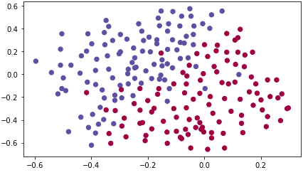
Each dot corresponds to a position on the football field where a football player has hit the ball with his/her head after the French goal keeper has shot the ball from the left side of the football field.
- If the dot is blue, it means the French player managed to hit the ball with his/her head
- If the dot is red, it means the other team's player hit the ball with their head
Your goal: Use a deep learning model to find the positions on the field where the goalkeeper should kick the ball.
CHAPTER 4. 'Non-Regularized Model'
You will use the following neural network (already implemented for you below). This model can be used:
- in regularization mode -- by setting the lambd input to a non-zero value. We use "lambd" instead of "lambda" because "lambda" is a reserved keyword in Python.
- in dropout mode -- by setting the keep_prob to a value less than one
You will first try the model without any regularization. Then, you will implement:
- L2 regularization -- functions: "compute_cost_with_regularization()" and "backward_propagation_with_regularization()"
- Dropout -- functions: "forward_propagation_with_dropout()" and "backward_propagation_with_dropout()"
In each part, you will run this model with the correct inputs so that it calls the functions you've implemented. Take a look at the code below to familiarize yourself with the model.
def model(X, Y, learning_rate = 0.3, num_iterations = 30000, print_cost = True, lambd = 0, keep_prob = 1):
    """
    Implements a three-layer neural network: LINEAR->RELU->LINEAR->RELU->LINEAR->SIGMOID.

    Arguments:
    X -- input data, of shape (input size, number of examples)
    Y -- true "label" vector (1 for blue dot / 0 for red dot), of shape (output size, number of examples)
    learning_rate -- learning rate of the optimization
    num_iterations -- number of iterations of the optimization loop
    print_cost -- If True, print the cost every 10000 iterations
    lambd -- regularization hyperparameter, scalar
    keep_prob - probability of keeping a neuron active during drop-out, scalar.

    Returns:
    parameters -- parameters learned by the model. They can then be used to predict.
    """

    grads = {}
    costs = []                            # to keep track of the cost
    m = X.shape[1]                        # number of examples
    layers_dims = [X.shape[0], 20, 3, 1]

    # Initialize parameters dictionary.
    parameters = initialize_parameters(layers_dims)

    # Loop (gradient descent)

    for i in range(0, num_iterations):

        # Forward propagation: LINEAR -> RELU -> LINEAR -> RELU -> LINEAR -> SIGMOID.
        if keep_prob == 1:
            a3, cache = forward_propagation(X, parameters)
        elif keep_prob < 1:
            a3, cache = forward_propagation_with_dropout(X, parameters, keep_prob)

        # Cost function
        if lambd == 0:
            cost = compute_cost(a3, Y)
        else:
            cost = compute_cost_with_regularization(a3, Y, parameters, lambd)

        # Backward propagation.
        assert (lambd == 0 or keep_prob == 1)   # it is possible to use both L2 regularization and dropout,
                                                # but this assignment will only explore one at a time
        if lambd == 0 and keep_prob == 1:
            grads = backward_propagation(X, Y, cache)
        elif lambd != 0:
            grads = backward_propagation_with_regularization(X, Y, cache, lambd)
        elif keep_prob < 1:
            grads = backward_propagation_with_dropout(X, Y, cache, keep_prob)

        # Update parameters.
        parameters = update_parameters(parameters, grads, learning_rate)

        # Print the loss every 10000 iterations
        if print_cost and i % 10000 == 0:
            print("Cost after iteration {}: {}".format(i, cost))
        if print_cost and i % 1000 == 0:
            costs.append(cost)

    # plot the cost
    plt.plot(costs)
    plt.ylabel('cost')
    plt.xlabel('iterations (x1,000)')
    plt.title("Learning rate =" + str(learning_rate))
    plt.show()

    return parameters
Let's train the model without any regularization, and observe the accuracy on the train/test sets.
parameters = model(train_X, train_Y)
print ("On the training set:")
predictions_train = predict(train_X, train_Y, parameters)
print ("On the test set:")
predictions_test = predict(test_X, test_Y, parameters)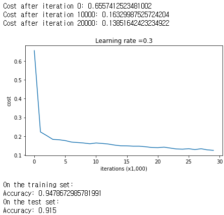
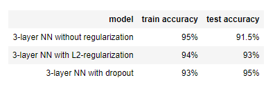
The train accuracy is 94.8% while the test accuracy is 91.5%. This is the baseline model (you will observe the impact of regularization on this model). Run the following code to plot the decision boundary of your model.
plt.title("Model without regularization")
axes = plt.gca()
axes.set_xlim([-0.75,0.40])
axes.set_ylim([-0.75,0.65])
plot_decision_boundary(lambda x: predict_dec(parameters, x.T), train_X, train_Y)

CHAPTER 5. 'L2 Regularization'
The standard way to avoid overfitting is called L2 regularization. It consists of appropriately modifying cost function.

# GRADED FUNCTION: compute_cost_with_regularization

def compute_cost_with_regularization(A3, Y, parameters, lambd):
    """
    Implement the cost function with L2 regularization. See formula (2) above.

    Arguments:
    A3 -- post-activation, output of forward propagation, of shape (output size, number of examples)
    Y -- "true" labels vector, of shape (output size, number of examples)
    parameters -- python dictionary containing parameters of the model

    Returns:
    cost - value of the regularized loss function (formula (2))
    """
    m = Y.shape[1]
    W1 = parameters["W1"]
    W2 = parameters["W2"]
    W3 = parameters["W3"]

    cross_entropy_cost = compute_cost(A3, Y) # This gives you the cross-entropy part of the cost

    #(≈ 1 lines of code)
    # L2_regularization_cost =
    # YOUR CODE STARTS HERE
    L2_regularization_cost = (1/m) * (lambd/2) * (np.sum(np.square(W1)) + np.sum(np.square(W2)) + np.sum(np.square(W3)))

    # YOUR CODE ENDS HERE

    cost = cross_entropy_cost + L2_regularization_cost

    return cost
A3, t_Y, parameters = compute_cost_with_regularization_test_case()
cost = compute_cost_with_regularization(A3, t_Y, parameters, lambd=0.1)
print("cost = " + str(cost))

compute_cost_with_regularization_test(compute_cost_with_regularization)
# GRADED FUNCTION: backward_propagation_with_regularization

def backward_propagation_with_regularization(X, Y, cache, lambd):
    """
    Implements the backward propagation of our baseline model to which we added an L2 regularization.

    Arguments:
    X -- input dataset, of shape (input size, number of examples)
    Y -- "true" labels vector, of shape (output size, number of examples)
    cache -- cache output from forward_propagation()
    lambd -- regularization hyperparameter, scalar

    Returns:
    gradients -- A dictionary with the gradients with respect to each parameter, activation and pre-activation variables
    """

    m = X.shape[1]
    (Z1, A1, W1, b1, Z2, A2, W2, b2, Z3, A3, W3, b3) = cache

    dZ3 = A3 - Y
    #(≈ 1 lines of code)
    # dW3 = 1./m * np.dot(dZ3, A2.T) + None
    # YOUR CODE STARTS HERE
    dW3 = 1./m * np.dot(dZ3, A2.T) + lambd/m * W3

    # YOUR CODE ENDS HERE
    db3 = 1. / m * np.sum(dZ3, axis=1, keepdims=True)

    dA2 = np.dot(W3.T, dZ3)
    dZ2 = np.multiply(dA2, np.int64(A2 > 0))
    #(≈ 1 lines of code)
    # dW2 = 1./m * np.dot(dZ2, A1.T) + None
    # YOUR CODE STARTS HERE
    dW2 = 1./m * np.dot(dZ2, A1.T) + lambd/m * W2

    # YOUR CODE ENDS HERE
    db2 = 1. / m * np.sum(dZ2, axis=1, keepdims=True)

    dA1 = np.dot(W2.T, dZ2)
    dZ1 = np.multiply(dA1, np.int64(A1 > 0))
    #(≈ 1 lines of code)
    # dW1 = 1./m * np.dot(dZ1, X.T) + None
    # YOUR CODE STARTS HERE
    dW1 = 1./m * np.dot(dZ1, X.T) + lambd/m * W1

    # YOUR CODE ENDS HERE
    db1 = 1. / m * np.sum(dZ1, axis=1, keepdims=True)

    gradients = {"dZ3": dZ3, "dW3": dW3, "db3": db3,"dA2": dA2,
                 "dZ2": dZ2, "dW2": dW2, "db2": db2, "dA1": dA1,
                 "dZ1": dZ1, "dW1": dW1, "db1": db1}

    return gradients
t_X, t_Y, cache = backward_propagation_with_regularization_test_case()

grads = backward_propagation_with_regularization(t_X, t_Y, cache, lambd = 0.7)
print ("dW1 = \n"+ str(grads["dW1"]))
print ("dW2 = \n"+ str(grads["dW2"]))
print ("dW3 = \n"+ str(grads["dW3"]))
backward_propagation_with_regularization_test(backward_propagation_with_regularization)

Let's now run the model with L2 regularization (𝜆=0.7)(λ=0.7). The model() function will call:
- compute_cost_with_regularization instead of compute_cost
- backward_propagation_with_regularization instead of backward_propagation
parameters = model(train_X, train_Y, lambd = 0.7)
print ("On the train set:")
predictions_train = predict(train_X, train_Y, parameters)
print ("On the test set:")
predictions_test = predict(test_X, test_Y, parameters)

plt.title("Model with L2-regularization")
axes = plt.gca()
axes.set_xlim([-0.75,0.40])
axes.set_ylim([-0.75,0.65])
plot_decision_boundary(lambda x: predict_dec(parameters, x.T), train_X, train_Y)
Observations:
- The value of 𝜆λ is a hyperparameter that you can tune using a dev set.
- L2 regularization makes your decision boundary smoother. If 𝜆λ is too large, it is also possible to "oversmooth", resulting in a model with high bias.
What is L2-regularization actually doing?:
L2-regularization relies on the assumption that a model with small weights is simpler than a model with large weights. Thus, by penalizing the square values of the weights in the cost function you drive all the weights to smaller values. It becomes too costly for the cost to have large weights! This leads to a smoother model in which the output changes more slowly as the input changes.
What you should remember: the implications of L2-regularization on:
- The cost computation:
- A regularization term is added to the cost.
- The backpropagation function:
- There are extra terms in the gradients with respect to weight matrices.
- Weights end up smaller ("weight decay"):
- Weights are pushed to smaller values.
CHAPTER 6. 'Dropout'
■ 6.1. Forward Propagation with Dropout
When you shut some neurons down, you actually modify your model. The idea behind drop-out is that at each iteration, you train a different model that uses only a subset of your neurons. With dropout, your neurons thus become less sensitive to the activation of one other specific neuron, because that other neuron might be shut down at any time.
Implement the forward propagation with dropout. You are using a 3 layer neural network, and will add dropout to the first and second hidden layers. We will not apply dropout to the input layer or output layer.
# GRADED FUNCTION: forward_propagation_with_dropout

def forward_propagation_with_dropout(X, parameters, keep_prob = 0.5):
    """
    Implements the forward propagation: LINEAR -> RELU + DROPOUT -> LINEAR -> RELU + DROPOUT -> LINEAR -> SIGMOID.

    Arguments:
    X -- input dataset, of shape (2, number of examples)
    parameters -- python dictionary containing your parameters "W1", "b1", "W2", "b2", "W3", "b3":
                    W1 -- weight matrix of shape (20, 2)
                    b1 -- bias vector of shape (20, 1)
                    W2 -- weight matrix of shape (3, 20)
                    b2 -- bias vector of shape (3, 1)
                    W3 -- weight matrix of shape (1, 3)
                    b3 -- bias vector of shape (1, 1)
    keep_prob - probability of keeping a neuron active during drop-out, scalar

    Returns:
    A3 -- last activation value, output of the forward propagation, of shape (1,1)
    cache -- tuple, information stored for computing the backward propagation
    """

    np.random.seed(1)

    # retrieve parameters
    W1 = parameters["W1"]
    b1 = parameters["b1"]
    W2 = parameters["W2"]
    b2 = parameters["b2"]
    W3 = parameters["W3"]
    b3 = parameters["b3"]

    # LINEAR -> RELU -> LINEAR -> RELU -> LINEAR -> SIGMOID
    Z1 = np.dot(W1, X) + b1
    A1 = relu(Z1)
    #(≈ 4 lines of code)         # Steps 1-4 below correspond to the Steps 1-4 described above.
    # D1 =                                           # Step 1: initialize matrix D1 = np.random.rand(..., ...)
    # D1 =                                           # Step 2: convert entries of D1 to 0 or 1 (using keep_prob as the threshold)
    # A1 =                                           # Step 3: shut down some neurons of A1
    # A1 =                                           # Step 4: scale the value of neurons that haven't been shut down
    # YOUR CODE STARTS HERE
    D1 = np.random.rand(A1.shape[0], A1.shape[1])
    D1 = (D1 < keep_prob).astype(int)
    A1 = np.multiply(D1, A1)
    A1 = A1/ keep_prob
    # YOUR CODE ENDS HERE

    Z2 = np.dot(W2, A1) + b2
    A2 = relu(Z2)
    #(≈ 4 lines of code)
    # D2 =                                           # Step 1: initialize matrix D2 = np.random.rand(..., ...)
    # D2 =                                           # Step 2: convert entries of D2 to 0 or 1 (using keep_prob as the threshold)
    # A2 =                                           # Step 3: shut down some neurons of A2
    # A2 =                                           # Step 4: scale the value of neurons that haven't been shut down
    # YOUR CODE STARTS HERE
    D2 = np.random.rand(A2.shape[0], A2.shape[1])
    D2 = (D2 < keep_prob).astype(int)
    A2 = np.multiply(D2, A2)
    A2 = A2/ keep_prob

    # YOUR CODE ENDS HERE
    Z3 = np.dot(W3, A2) + b3
    A3 = sigmoid(Z3)

    cache = (Z1, D1, A1, W1, b1, Z2, D2, A2, W2, b2, Z3, A3, W3, b3)

    return A3, cache
t_X, parameters = forward_propagation_with_dropout_test_case()

A3, cache = forward_propagation_with_dropout(t_X, parameters, keep_prob=0.7)
print ("A3 = " + str(A3))

forward_propagation_with_dropout_test(forward_propagation_with_dropout)
■ 6.2. Backward Propagation with Dropout
Implement the backward propagation with dropout. As before, you are training a 3 layer network. Add dropout to the first and second hidden layers, using the masks 𝐷[1] and 𝐷[2] stored in the cache.
# GRADED FUNCTION: backward_propagation_with_dropout

def backward_propagation_with_dropout(X, Y, cache, keep_prob):
    """
    Implements the backward propagation of our baseline model to which we added dropout.

    Arguments:
    X -- input dataset, of shape (2, number of examples)
    Y -- "true" labels vector, of shape (output size, number of examples)
    cache -- cache output from forward_propagation_with_dropout()
    keep_prob - probability of keeping a neuron active during drop-out, scalar

    Returns:
    gradients -- A dictionary with the gradients with respect to each parameter, activation and pre-activation variables
    """

    m = X.shape[1]
    (Z1, D1, A1, W1, b1, Z2, D2, A2, W2, b2, Z3, A3, W3, b3) = cache

    dZ3 = A3 - Y
    dW3 = 1./m * np.dot(dZ3, A2.T)
    db3 = 1./m * np.sum(dZ3, axis=1, keepdims=True)
    dA2 = np.dot(W3.T, dZ3)
    #(≈ 2 lines of code)
    # dA2 =                # Step 1: Apply mask D2 to shut down the same neurons as during the forward propagation
    # dA2 =                # Step 2: Scale the value of neurons that haven't been shut down
    # YOUR CODE STARTS HERE
    dA2 = np.multiply(dA2, D2)
    dA2 = dA2 / keep_prob

    # YOUR CODE ENDS HERE
    dZ2 = np.multiply(dA2, np.int64(A2 > 0))
    dW2 = 1./m * np.dot(dZ2, A1.T)
    db2 = 1./m * np.sum(dZ2, axis=1, keepdims=True)

    dA1 = np.dot(W2.T, dZ2)
    #(≈ 2 lines of code)
    # dA1 =                # Step 1: Apply mask D1 to shut down the same neurons as during the forward propagation
    # dA1 =                # Step 2: Scale the value of neurons that haven't been shut down
    # YOUR CODE STARTS HERE
    dA1 = np.multiply(dA1, D1)
    dA1 = dA1 / keep_prob

    # YOUR CODE ENDS HERE
    dZ1 = np.multiply(dA1, np.int64(A1 > 0))
    dW1 = 1./m * np.dot(dZ1, X.T)
    db1 = 1./m * np.sum(dZ1, axis=1, keepdims=True)

    gradients = {"dZ3": dZ3, "dW3": dW3, "db3": db3,"dA2": dA2,
                 "dZ2": dZ2, "dW2": dW2, "db2": db2, "dA1": dA1,
                 "dZ1": dZ1, "dW1": dW1, "db1": db1}

    return gradients
t_X, t_Y, cache = backward_propagation_with_dropout_test_case()

gradients = backward_propagation_with_dropout(t_X, t_Y, cache, keep_prob=0.8)

print ("dA1 = \n" + str(gradients["dA1"]))
print ("dA2 = \n" + str(gradients["dA2"]))

backward_propagation_with_dropout_test(backward_propagation_with_dropout)

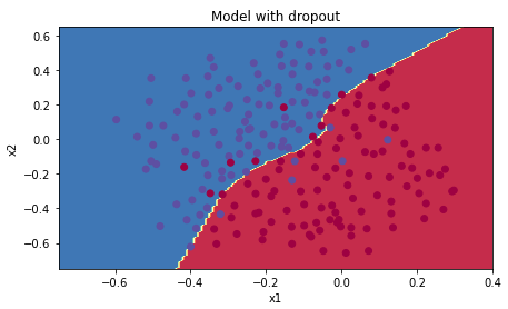
Let's now run the model with dropout (keep_prob = 0.86). It means at every iteration you shut down each neurons of layer 1 and 2 with 14% probability. The function model() will now call:
parameters = model(train_X, train_Y, keep_prob = 0.86, learning_rate = 0.3)

print ("On the train set:")
predictions_train = predict(train_X, train_Y, parameters)
print ("On the test set:")
predictions_test = predict(test_X, test_Y, parameters)

Dropout works great! The test accuracy has increased again (to 95%)! Your model is not overfitting the training set and does a great job on the test set. The French football team will be forever grateful to you!
Run the code below to plot the decision boundary.
plt.title("Model with dropout")
axes = plt.gca()
axes.set_xlim([-0.75,0.40])
axes.set_ylim([-0.75,0.65])
plot_decision_boundary(lambda x: predict_dec(parameters, x.T), train_X, train_Y)
What you should remember about dropout:
- Dropout is a regularization technique.
- You only use dropout during training. Don't use dropout (randomly eliminate nodes) during test time.
- Apply dropout both during forward and backward propagation.
- During training time, divide each dropout layer by keep_prob to keep the same expected value for the activations. For example, if keep_prob is 0.5, then we will on average shut down half the nodes, so the output will be scaled by 0.5 since only the remaining half are contributing to the solution. Dividing by 0.5 is equivalent to multiplying by 2. Hence, the output now has the same expected value. You can check that this works even when keep_prob is other values than 0.5.
CHAPTER 7. 'Conclusions'
Note that regularization hurts training set performance! This is because it limits the ability of the network to overfit to the training set. But since it ultimately gives better test accuracy, it is helping your system.
What we want you to remember from this notebook:
- Regularization will help you reduce overfitting.
- Regularization will drive your weights to lower values.
- L2 regularization and Dropout are two very effective regularization techniques.
■ 마무리
"Improving Deep Neural Networks" (Andrew Ng)의 1주차 "Regularization"의 실습에 대해서 정리해봤습니다.
그럼 오늘 하루도 즐거운 나날 되길 기도하겠습니다
좋아요와 댓글 부탁드립니다 :)
감사합니다.
'COURSERA' 카테고리의 다른 글
| week 2_Optimization Algorithms (Andrew Ng) (0) | 2022.02.20 |
|---|---|
| week 1_Gradient Checking 실습 (Andrew Ng) (0) | 2022.02.18 |
| week 1_Initialization 실습 (Andrew Ng) (0) | 2022.02.18 |
| week 1_Practical Aspects of Deep Learning 연습문제 (Andrew Ng) (0) | 2022.02.18 |
| week 1_Setting up optimization problem (Andrew Ng) (0) | 2022.02.18 |


댓글